Aggregate Expenditure and Equilibrium Output: Core Concepts in Macroeconomics

Aggregate Expenditure and Equilibrium Output

Introduction to Aggregate Expenditure

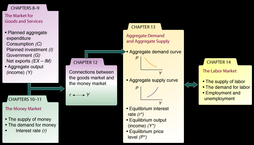
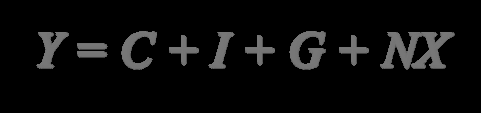
Aggregate expenditure is a fundamental concept in macroeconomics, representing the total planned spending in an economy during a given period. It is composed of consumption, investment, government spending, and net exports. Understanding aggregate expenditure is crucial for analyzing how economies achieve equilibrium output and income.

• Aggregate planned expenditure = Consumption (C) + Planned Investment (I) + Government Expenditure (G) + Exports (X) - Planned Imports (M)

• Real GDP may differ from aggregate planned expenditure due to unplanned changes in inventories.

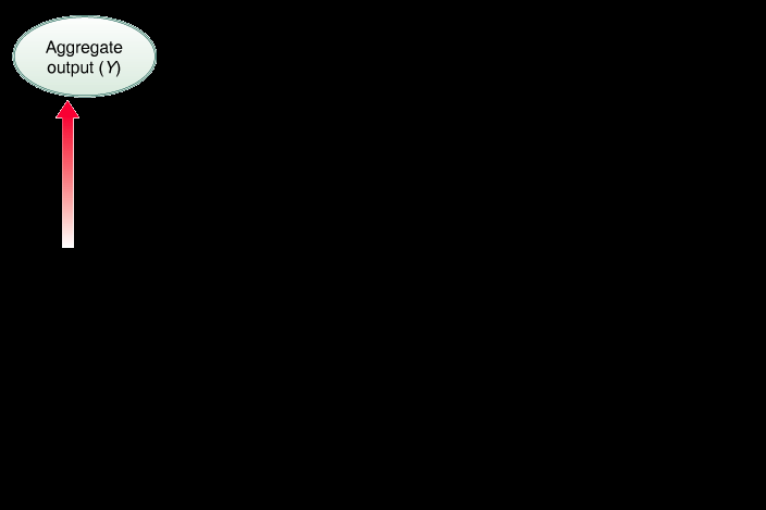
• Aggregate income (output) is the sum of all income received by factors of production (wages, rents, interest, profits).

Aggregate Output and Planned Expenditure

In a closed economy without government, aggregate output (Y) and planned aggregate expenditure (AE) are central to determining equilibrium. Equilibrium occurs when output equals planned expenditure, meaning there is no tendency for change.

• Equilibrium condition: $Y = AE$ or $Y = C + I$

• Saving (S): The portion of income not consumed. $Y \equiv C + S$ and $S \equiv Y - C$

• Identity: An equation always true by definition.

Income, Consumption, and Saving

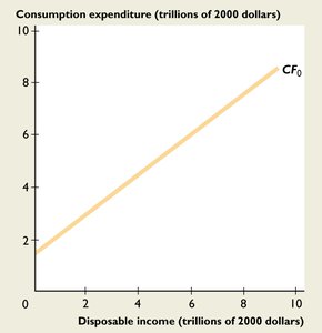
The Consumption Function

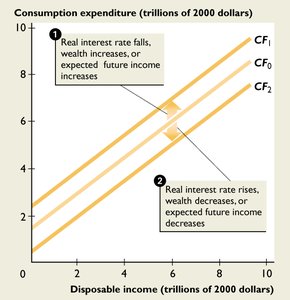
The consumption function describes the relationship between consumption expenditure and income. It is typically linear, with a positive slope indicating that as income rises, consumption increases.

• Marginal Propensity to Consume (MPC): Fraction of a change in income spent on consumption. $MPC = \frac{\Delta C}{\Delta Y}$

• Aggregate consumption function: $C = a + bY$, where $a$ is autonomous consumption and $b$ is the MPC.

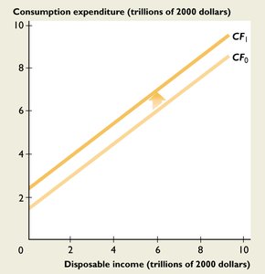
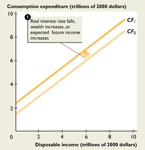
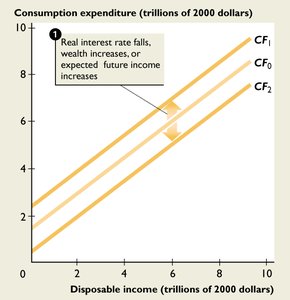
• Factors influencing consumption: Income, real interest rate, wealth, expected future income.

The Saving Function

The saving function shows the relationship between saving and income. The marginal propensity to save (MPS) is the fraction of a change in income that is saved.

• Marginal Propensity to Save (MPS): $MPS = \frac{\Delta S}{\Delta Y}$

• Saving function: $S = Y - C$

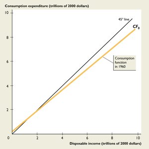
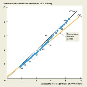
Empirical Consumption Functions

Empirical data can be used to estimate consumption functions for different periods, showing how consumption patterns change over time due to shifts in economic factors.

• Example: U.S. consumption function in the 1960s vs. 2000s.

• The slope of the consumption function (MPC) can change as economic conditions evolve.

Planned Investment and Aggregate Expenditure

Investment Concepts

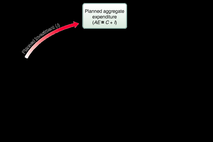
Investment refers to purchases by firms of new buildings, equipment, and additions to inventories. Planned investment is what firms intend to invest, while actual investment includes unplanned changes in inventories.

• Planned aggregate expenditure (AE): Total amount the economy plans to spend in a period. $AE \equiv C + I$

• Actual vs. planned investment: Actual investment includes unplanned inventory changes.

Equilibrium Output and the Multiplier

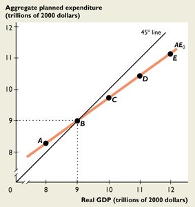
Equilibrium Output

Equilibrium output is achieved when planned aggregate expenditure equals aggregate output. This can be analyzed using both the expenditure and saving/investment approaches.

• Equilibrium condition: $Y = AE$

• S = I approach: Only when planned investment equals saving will equilibrium occur.

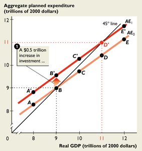
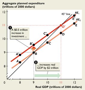
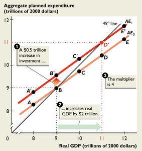
The Multiplier Effect

The multiplier is the ratio of the change in equilibrium output to a change in an autonomous variable, such as investment. It explains how initial increases in spending lead to larger increases in output.

• Multiplier formula: $Multiplier = \frac{\text{Change in equilibrium expenditure}}{\text{Change in autonomous expenditure}}$

• Relationship to MPC: $\Delta Y = \Delta C + \Delta I$ and $\Delta C = MPC \times \Delta Y$

• Substituting gives: $\Delta Y = MPC \times \Delta Y + \Delta I$

• Rearranged: $(1 - MPC) \times \Delta Y = \Delta I$

• Final multiplier: $\Delta Y = \frac{\Delta I}{1 - MPC}$

• When $MPC = 0.75$, multiplier is $\frac{1}{1 - 0.75} = 4$

Multiplier in the Real World

In practice, the multiplier is often smaller than theoretical values due to leakages and other economic factors. For example, a sustained increase in autonomous spending of $10 billion may raise real GDP by about $20 billion.

• Real-world multiplier: Typically around 2 for the U.S. economy.

Summary Table: Consumption and Equilibrium Output

The following table illustrates the relationship between aggregate output, consumption, planned investment, aggregate expenditure, unplanned inventory changes, and equilibrium status.

Aggregate Output (Y)	Aggregate Consumption (C)	Planned Investment (I)	Planned Aggregate Expenditure (AE = C + I)	Unplanned Inventory Change (Y - AE)	Equilibrium? (Y = AE?)
100	175	25	200	-100	No
200	250	25	275	-75	No
400	400	25	425	-25	No
500	475	25	500	0	Yes
600	550	25	575	+25	No
800	700	25	725	+75	No
1,000	850	25	875	+125	No

Key Equations and Definitions

• Aggregate Output: $Y = C + I + G + NX$

• Consumption Function: $C = a + bY$

• Saving Function: $S = Y - C$

• Multiplier: $\frac{1}{1 - MPC}$

Example Problems

1. Given $C = 200 + 0.8Y$, derive the saving function and write out the algebraic representation.

2. In a two-sector economy where $C = 100 + 0.9Y$ and $I = 50$, calculate the equilibrium level of output. What would the level of consumption be if the economy were operating at $Y = 1400$? What would be the amount of unplanned investment at this level? In which direction would you expect the economy to move at $Y = 1400$ and why?

Additional info: The notes have been expanded to include definitions, formulas, and examples for clarity and completeness, as well as relevant images and a summary table for exam preparation.