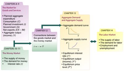
Aggregate Expenditure and Equilibrium Output: ch 8

Aggregate Expenditure and Equilibrium Output

Introduction to Aggregate Expenditure

Aggregate expenditure (AE) is a foundational concept in macroeconomics, representing the total planned spending in an economy during a specific period. It is the sum of consumption, planned investment, government expenditure, and net exports. The equilibrium output is achieved when aggregate output (income) equals aggregate planned expenditure.

• Aggregate Planned Expenditure (AE): $AE = C + I + G + NX$

• Aggregate Output (Y): The total value of goods and services produced, equivalent to aggregate income.

• Equilibrium Condition: $Y = AE$

Income, Consumption, and Saving

Definitions and Relationships

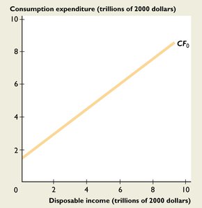
Household income can be either consumed or saved. The consumption function describes the relationship between consumption and income, while the saving function captures the portion of income not spent.

• Consumption Function: $C = a + bY$ where $a$ is autonomous consumption and $b$ is the marginal propensity to consume (MPC).

• Saving Function: $S = Y - C$

• Marginal Propensity to Consume (MPC): The fraction of additional income spent on consumption. $MPC = \frac{\Delta C}{\Delta Y}$

• Marginal Propensity to Save (MPS): The fraction of additional income saved. $MPS = \frac{\Delta S}{\Delta Y}$

• Identity: $Y \equiv C + S$

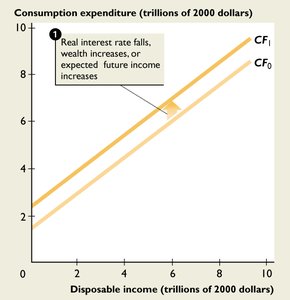
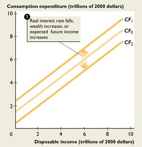
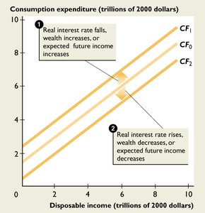
Shifts in the Consumption Function

The consumption function can shift due to changes in factors other than income, such as the real interest rate, wealth, and expected future income. An upward shift indicates increased consumption at every income level.

• Factors Influencing Consumption:

  • Income

  • Real interest rate

  • Wealth

  • Expected future income

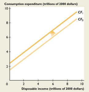
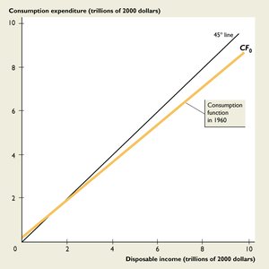
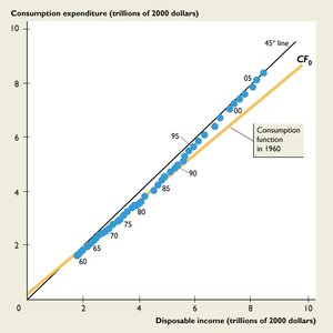
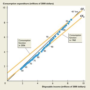
The U.S. Consumption Function: Historical Perspective

Empirical data from the United States demonstrates how the consumption function has shifted over time, reflecting changes in economic conditions and consumer behavior.

• CF0: Consumption function estimate for the 1960s

• CF1: Consumption function estimate for the 2000s

• Slope (MPC): For the U.S., the MPC has been estimated at 0.87 in recent decades.

Planned Investment and Actual Investment

Definitions

Investment in macroeconomics refers to purchases by firms of new capital goods and additions to inventories. Planned investment is what firms intend to invest, while actual investment includes unplanned changes in inventories.

• Planned Investment (I): Additions to capital stock and inventory that are planned by firms.

• Actual Investment: The actual amount of investment, including unplanned inventory changes.

• Change in Inventory: Production minus sales.

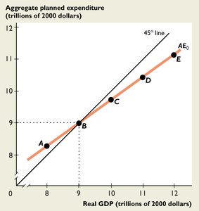
Equilibrium Aggregate Output (Income)

Determining Equilibrium

Equilibrium occurs when planned aggregate expenditure equals aggregate output (income). At this point, there is no tendency for change, and unplanned inventory changes are zero.

• Equilibrium Condition: $Y = AE$

• Alternative Approach: Equilibrium also occurs when planned saving equals planned investment ($S = I$).

Aggregate Output (Y)	Aggregate Consumption (C)	Planned Investment (I)	Planned Aggregate Expenditure (AE)	Unplanned Inventory Change	Equilibrium?
100	175	25	200	-100	No
200	250	25	275	-75	No
400	400	25	425	-25	No
500	475	25	500	0	Yes
600	550	25	575	+25	No
800	700	25	725	+75	No
1,000	850	25	875	+125	No

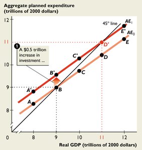
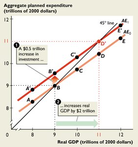
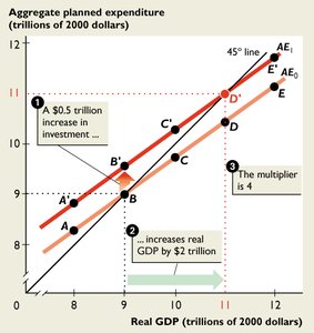
The Multiplier Effect

Concept and Calculation

The multiplier measures how a change in autonomous expenditure (such as investment) leads to a larger change in equilibrium output. The size of the multiplier depends on the marginal propensity to consume (MPC).

• Multiplier Formula: $\text{Multiplier} = \frac{1}{1 - MPC}$

• Change in Output: $\Delta Y = \frac{\Delta I}{1 - MPC}$

• Example: If $MPC = 0.75$, then $\text{Multiplier} = 4$

Multiplier in the Real World

In practice, the multiplier is often smaller than the theoretical value due to leakages such as taxes, imports, and savings. In the U.S., a sustained increase in autonomous spending of $10 billion typically raises real GDP by about $20 billion, implying a multiplier of about 2.

Practice Questions

1. Assume a consumption function of the form $C = 200 + 0.8Y$. Derive the saving function and write out the algebraic representation.

2. Assume a two-sector economy where $C = 100 + 0.9Y$ and $I = 50$. Calculate the equilibrium level of output for this hypothetical economy. What would the level of consumption be if the economy were operating at 1400? What would be the amount of unplanned investment at this level? In which direction would you expect the economy to move to at $1400$ and why?