Aggregate Expenditure and Output in the Short Run: Study Notes

Aggregate Expenditure and Output in the Short Run

The Aggregate Expenditure Model

The aggregate expenditure (AE) model is a foundational macroeconomic framework that analyzes the short-run relationship between total spending and real GDP, under the assumption that the price level is constant. Developed by John Maynard Keynes, this model helps explain why economies experience fluctuations such as recessions and expansions.

• Aggregate Expenditure (AE): The total spending in the economy, comprising consumption (C), planned investment (I), government purchases (G), and net exports (NX).

• Macroeconomic Equilibrium: Occurs when aggregate expenditure equals GDP, i.e., $AE = GDP$.

• Adjustment Mechanism: If AE > GDP, inventories fall and GDP rises; if AE < GDP, inventories rise and GDP falls. Equilibrium is achieved when AE = GDP.

Formula:

$AE = C + I + G + NX$

Actual Investment: $\text{Actual Investment} = \text{Planned Investment} + \text{Unplanned Change in Inventories}$

Components of Aggregate Expenditure

Keynes identified four main components of aggregate expenditure:

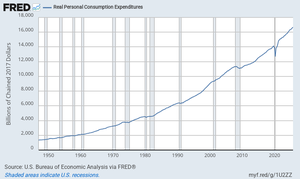
• Consumption (C): Household spending on goods and services.

• Planned Investment (I): Firm spending on capital goods and household spending on new homes.

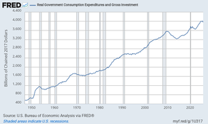
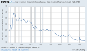
• Government Purchases (G): Government spending on goods and services (excluding transfers).

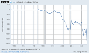
• Net Exports (NX): Exports minus imports.

Determinants of Consumption

Consumption is influenced by several variables:

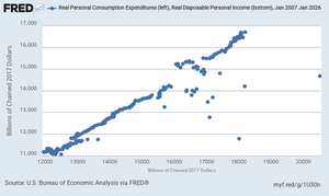
• Current Disposable Income (YD): $YD = Y - T$ (income after taxes and transfers).

• Household Wealth: Value of assets minus liabilities; increases in wealth raise consumption.

• Expected Future Income: Households smooth consumption based on expectations.

• Price Level: Higher prices reduce real wealth and consumption.

• Interest Rate: Higher real interest rates discourage consumption, especially of durable goods.

The Consumption Function and Marginal Propensities

The consumption function expresses the relationship between consumption and disposable income:

• Consumption Function: $C = a + bY_D$, where $a$ is autonomous consumption and $b$ is the marginal propensity to consume (MPC).

• Marginal Propensity to Consume (MPC): The change in consumption from an additional dollar of income.

• Marginal Propensity to Save (MPS): The change in saving from an additional dollar of income. $MPC + MPS = 1$.

Example: If $MPC = 0.91$, a $10$billion increase in disposable income increases consumption by $9.1$ billion.

Determinants of Investment, Government Purchases, and Net Exports

• Investment (I): Determined by expectations of future profitability, real interest rate, corporate taxes, and cash flow.

• Government Purchases (G): Includes all government spending on goods and services, excluding transfers.

• Net Exports (NX): Influenced by the U.S. price level relative to other countries, exchange rates, and relative GDP growth rates.

Summary Table: Factors Affecting Aggregate Expenditure

Component	Main Determinants
Consumption (C)	Disposable income, wealth, expected future income, price level, interest rate
Investment (I)	Future profitability, interest rate, corporate taxes, cash flow
Government Purchases (G)	Government policy decisions
Net Exports (NX)	Relative price levels, exchange rates, relative GDP growth

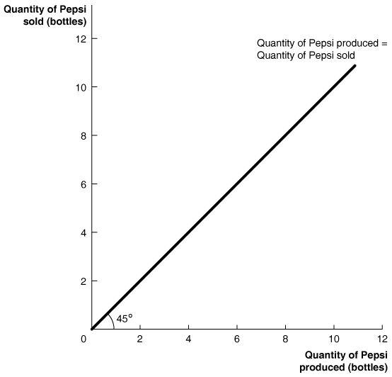
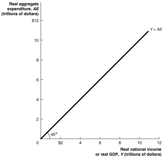
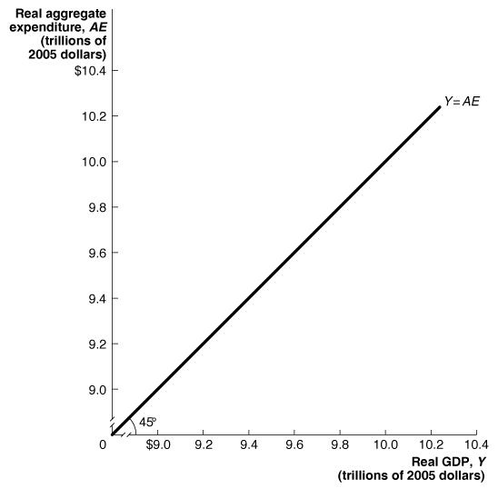
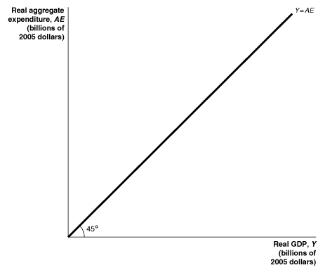
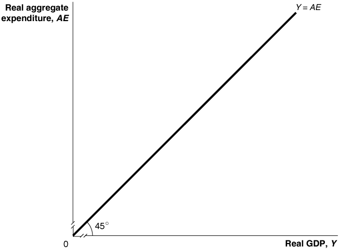
Graphing Macroeconomic Equilibrium: The 45°-Line Diagram

The 45°-line diagram (Keynesian cross) is a graphical tool to illustrate macroeconomic equilibrium, where every point on the 45° line represents equality between aggregate expenditure and GDP.

• Points above the line: AE > GDP (inventories fall, GDP rises)

• Points below the line: AE < GDP (inventories rise, GDP falls)

• Equilibrium: Where the AE line crosses the 45° line

The Multiplier Effect

The multiplier effect describes how an initial change in autonomous expenditure leads to a larger change in equilibrium GDP. This occurs because each round of spending induces further rounds of consumption.

• Multiplier Formula: $\text{Multiplier} = \frac{1}{1 - MPC}$

• Total Change in GDP: $\Delta Y = \text{Multiplier} \times \Delta \text{Autonomous Expenditure}$

• The larger the MPC, the larger the multiplier.

Example: If $MPC = 0.75$, a $100$increase in autonomous expenditure increases GDP by $100 \times 4 = $400$.

The Multiplier in Reverse: The Great Depression

A decrease in autonomous expenditure can also lead to a multiplied decrease in GDP, as seen during the Great Depression. The multiplier effect magnified reductions in spending, causing a severe economic downturn.

The Aggregate Demand Curve

The aggregate demand (AD) curve shows the inverse relationship between the price level and the level of planned aggregate expenditure (and thus real GDP), holding other factors constant.

• As the price level rises, AE falls, and equilibrium GDP decreases.

• As the price level falls, AE rises, and equilibrium GDP increases.

• Reasons: Wealth effect, interest rate effect, and international trade effect.

Algebra of Macroeconomic Equilibrium

Equilibrium GDP can be calculated using the following system of equations:

• $C = \bar{C} + MPC \cdot Y$

• $I = \bar{I}$

• $G = \bar{G}$

• $NX = \overline{NX}$

• $Y = C + I + G + NX$

Solving for equilibrium GDP:

$Y = \frac{\bar{C} + \bar{I} + \bar{G} + \overline{NX}}{1 - MPC}$

This formula shows that equilibrium GDP is determined by autonomous expenditure and the multiplier.

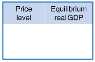
Summary Table: Price Level and Equilibrium GDP

Price level	Equilibrium real GDP
97	$10.2$ trillion
100	$10.0$ trillion
103	$9.8$ trillion

Key Takeaways

• Aggregate expenditure determines short-run GDP.

• Macroeconomic equilibrium occurs when AE = GDP.

• The multiplier effect amplifies changes in autonomous expenditure.

• The aggregate demand curve links price level changes to changes in equilibrium GDP via aggregate expenditure.