Aggregate Expenditure and Output in the Short Run: Study Notes

Aggregate Expenditure and Output in the Short Run

Introduction

This chapter explores the short-run relationship between total spending (aggregate expenditure) and real GDP, focusing on the Keynesian income-expenditure approach. The aggregate expenditure model is central to understanding how fluctuations in spending drive business cycles and macroeconomic equilibrium.

The Aggregate Expenditure Model

Definition and Components

• Aggregate Expenditure (AE): Total spending in the economy, defined as the sum of consumption (C), planned investment (I), government purchases (G), and net exports (NX).

• Formula: $AE = C + I + G + NX$

• Keynesian Model: Assumes the price level is constant in the short run, so changes in AE directly affect real GDP.

Macroeconomic Equilibrium: Occurs where aggregate expenditure equals GDP ($AE = GDP$). At this point, firms sell exactly what they produce, and inventories remain unchanged.

Planned vs. Actual Investment

• Inventories: Goods produced but not yet sold. Unplanned changes in inventories signal disequilibrium.

• Actual Investment > Planned Investment: Occurs when inventories rise unexpectedly (AE < GDP).

• Actual Investment < Planned Investment: Occurs when inventories fall unexpectedly (AE > GDP).

Adjustments to Equilibrium

• If AE > GDP: Inventories fall, firms increase production, GDP rises.

• If AE < GDP: Inventories rise, firms decrease production, GDP falls.

• Equilibrium is restored when AE = GDP.

Determinants of Aggregate Expenditure

Consumption (C)

• Key Determinants:

  1. Current disposable income

  2. Household wealth

  3. Expected future income

  4. The price level

  5. The interest rate

• Consumption Function: Relationship between consumption and disposable income.

• Marginal Propensity to Consume (MPC): The change in consumption from a change in disposable income. $MPC = \frac{\Delta C}{\Delta Y_D}$

• Marginal Propensity to Save (MPS): The change in saving from a change in disposable income. $MPS = 1 - MPC$

Investment (I)

• Key Determinants:

  1. Expectations of future profitability

  2. Interest rate

  3. Taxes (corporate income tax, investment tax incentives)

  4. Cash flow (difference between cash revenues and cash spending)

Government Purchases (G)

• All spending by federal, state, and local governments on goods and services.

Net Exports (NX)

• Key Determinants:

  1. Relative price levels (domestic vs. foreign)

  2. Relative GDP growth rates

  3. Exchange rates

Graphing Macroeconomic Equilibrium

The 45°-Line Diagram

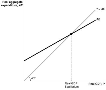
The 45°-line diagram is a graphical tool to illustrate macroeconomic equilibrium. The 45° line represents all points where AE equals real GDP. The intersection of the AE line with the 45° line indicates equilibrium GDP.

• Points above the 45° line: AE > GDP (inventories fall, GDP rises)

• Points below the 45° line: AE < GDP (inventories rise, GDP falls)

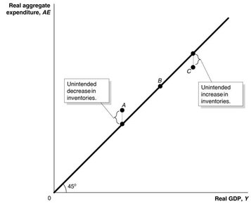
Unintended Inventory Changes

Unplanned changes in inventories indicate disequilibrium. If AE is greater than GDP, inventories decrease; if AE is less than GDP, inventories increase. The vertical distance between the AE line and the 45° line at any level of GDP shows the unplanned change in inventories.

The Multiplier Effect

Definition and Formula

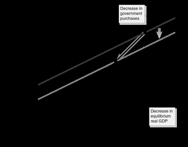
• Multiplier: The ratio of the change in equilibrium real GDP to the initial change in autonomous expenditure.

• Formula: $Multiplier = \frac{1}{1 - MPC}$

• Multiplier Effect: An autonomous change in expenditure leads to a larger change in equilibrium GDP due to induced increases in consumption.

Key Points about the Multiplier

• Occurs for both increases and decreases in autonomous expenditure.

• The larger the MPC, the larger the multiplier.

• The simple multiplier formula ignores real-world factors (imports, taxes, inflation, interest rates), so it overstates the actual multiplier.

The Paradox of Thrift

• If households simultaneously increase saving and reduce spending, aggregate expenditure and real GDP fall, potentially making households worse off in the short run.

The Aggregate Demand Curve

Relationship to Aggregate Expenditure

• Aggregate Demand (AD) Curve: Shows the relationship between the price level and the level of planned aggregate expenditure, holding other factors constant.

• There is an inverse relationship between the price level and aggregate expenditure due to:

  1. Wealth effect (changes in real value of household wealth)

  2. International trade effect (relative price levels affect net exports)

  3. Interest rate effect (higher prices increase money demand, raising interest rates and reducing investment)

Appendix: Algebra of Macroeconomic Equilibrium

Equilibrium Calculation

• General equilibrium condition: $Y = C + I + G + NX$

• With linear consumption function: $C = \overline{C} + MPC \cdot Y$

• Solving for equilibrium GDP: $Y = \frac{\overline{C} + \overline{I} + \overline{G} + \overline{NX}}{1 - MPC}$

• All terms in the numerator are autonomous expenditures.

Example: If $\overline{C} = 1,000$, $\overline{I} = 1,500$, $\overline{G} = 1,500$, $\overline{NX} = -500$, and $MPC = 0.65$: $Y = \frac{1,000 + 1,500 + 1,500 - 500}{1 - 0.65} = \frac{3,500}{0.35} = 10,000$

Summary Table: Key Formulas and Relationships

Concept	Formula	Description
Aggregate Expenditure	$AE = C + I + G + NX$	Total spending in the economy
Macroeconomic Equilibrium	$AE = GDP$	Equilibrium when spending equals output
Marginal Propensity to Consume	$MPC = \frac{\Delta C}{\Delta Y_D}$	Change in consumption per change in disposable income
Marginal Propensity to Save	$MPS = 1 - MPC$	Change in saving per change in disposable income
Multiplier	$\frac{1}{1 - MPC}$	Effect of autonomous expenditure on GDP
Equilibrium GDP	$Y = \frac{\overline{C} + \overline{I} + \overline{G} + \overline{NX}}{1 - MPC}$	GDP at equilibrium

Additional info: Real-world complications such as taxes, imports, and inflation reduce the size of the multiplier compared to the simple model. The aggregate expenditure model is most useful for understanding short-run fluctuations and cyclical unemployment, but not long-run growth or inflation.