Aggregate Expenditure and Output in the Short Run: Study Notes

Aggregate Expenditure and Output in the Short Run

Introduction

This chapter explores the aggregate expenditure model, a foundational concept in macroeconomics that explains the short-run relationship between total spending and real GDP, assuming a constant price level. The model is essential for understanding how economies reach equilibrium and how changes in spending affect output and employment.

The Aggregate Expenditure Model

Definition and Components

The aggregate expenditure model focuses on the short-run determination of total output in an economy. It assumes the price level is constant and examines how total spending (aggregate expenditure) determines real GDP.

• Adjusted for inflation. Total spending (total expenditures)

• Consumption (C): Household spending on goods and services.

• Planned Investment (I): Firm spending on capital goods and household spending on new homes (excludes unplanned inventory changes).

• Government Purchases (G): All levels of government spending on goods and services.

• Net Exports (NX): Exports minus imports.

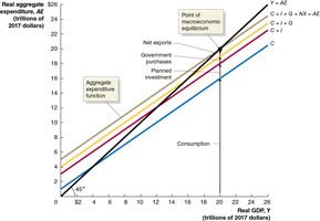
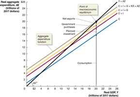
Aggregate expenditure (AE) is the sum of these four components: $AE = C + I + G + NX$

• The Toal spending in the economy

Planned vs. Actual Investment

Planned investment excludes unplanned changes in inventories, while actual investment includes them. Macroeconomic equilibrium occurs when planned investment equals actual investment, meaning there are no unplanned inventory changes.

Planned investment = Actual Investment - unplanned change in inventories

• The BEA measures actual investment, we will assume that their measurement is close enough to planned investment to use in our estimates of aggregate expenditures

Determinants of Aggregate Expenditure

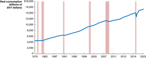
Real Consumption, 1979-2023

Consumption

Consumption is the largest component of aggregate expenditure and is influenced by several factors:

• Current Disposable Income (YD): Higher income leads to higher consumption.

YD = Y - T + TR

Current Disposable Income = Personal income - Personal income taxes +transfer payments

• Household Wealth: More wealth (assets, like homes, stocks and bonds, and bank accounts) increases consumption; a $1,000 increase in wealth typically raises annual consumption by $40–$50.

Household Wealth =Assets - Liabilities

• Expected Future Income: Households prefer to keep their consumption fairly stable from year to year even if their income fluctuates a lot from year to year. Consumption relates both to current and future income.

• Price Level: Higher prices reduce real wealth and consumption.

• Interest Rate: Higher real interest rates encourage saving and rather than spending, especially of durable goods.

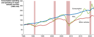
• Household spending on all consumption goods (blue line) is less volatile than spending on consumer durables like motor vehicles (cars and trucks) or recreational vehicles (RVs).

Volatility of Durable Goods Consumption

• Durable goods purchases are more volatile due to:

  1. Durable goods are long-lived: households can postpone buying them when incomes are down

  2. Goods substitutes exists- like used cars/RVs

  3. High prices make them risky purchases- the risk of not being able to pay back loans during times of uncertainty

  4. Pent-up demand typically follows a recession- purchases postponed during a recession will eventually be made

  5. Interest rates fluctuate- rising late in an expansion (discourages large purchases) and falling after a recession (encouraging those purchases)

The Consumption Function and Marginal Propensity to Consume (MPC)

The consumption function describes the relationship between consumption and disposable income. The marginal propensity to consume (MPC) is the change in consumption from an additional dollar of income.

$MPC = \frac{\Delta C}{\Delta Y}$

Consumption and National Income

• The distinction between these is relatively minor. So for this simple model, we will assume they are equal.

Disposable income (YD) = national income (Y) - net taxes (T-TR)

• Net taxes = taxes (T) - transfer payments (TR)

So...

National income = GDP = Disposable income (YD) + Net taxes (T-TR)

• If we assume that net taxes do not change as national income changes, we have the result that any change in disposable income is the same as the change in national income.

• MPC = c

Marginal Propensity to Save (MPS)

The marginal propensity to save (MPS) is the change in saving from an additional dollar of income. By definition:

$MPC + MPS = 1$

Investment

Investment is more volatile than consumption and is influenced by:

• Expectations of Future Profitability: Optimism increases investment; pessimism reduces it.

• Interest Rate: Business investment is often financed by borrowing: higher rates decrease investment; lower rates increase it.

• Taxes: Higher corporate taxes reduce investment; tax incentives increase it.

• Cash Flow: Firms with higher profits (own cash flow) can invest more.

• Cash flow= cash revenue received by a firm - cash spending by the firm

• Large contributor to cash flow is profit

• Unlike consumption, investment has not increased smoothly

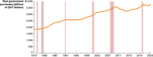
Government Purchases

Government purchases include all levels of government spending on goods and services (excluding transfer payments). They generally increase over time but can fluctuate due to policy changes or economic conditions.

Net Exports

Net exports are affected by:

• Price level in United States versus. the price level in other countries

• U.S. growth rate versus. growth rate in other countries (GDP)

• U.S. dollar exchange rate

U.S. net exports have been negative for decades, typically rising (becoming less negative) during recessions as imports fall.

• 

• If U.S GDP grows faster than foreign GDP, this means that Americans are experiencing higher incomes

Graphing Macroeconomic Equilibrium

The 45-Degree Line Diagram

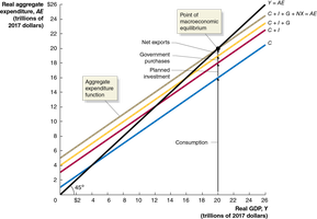
The 45-degree line diagram (Keynesian cross) is used to illustrate macroeconomic equilibrium, where aggregate expenditure equals real GDP. Any point on the 45-degree line represents equilibrium.

• Suppose in the whole economy there is a single product: Pepsi.

• For the Pepsi economy to be in equilibrium, the amount of Pepsi produced must equal the amount of Pepsi sold. Otherwise, inventories of Pepsi rise or fall.

PAGE 37

Finding Equilibrium

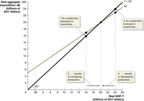
Equilibrium occurs where the aggregate expenditure function intersects the 45-degree line. If aggregate expenditure is above GDP, inventories fall and firms increase production. If below, inventories rise and firms cut production.

Recessionary Gaps

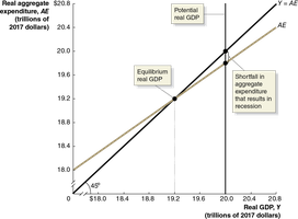
If equilibrium occurs below potential GDP, the economy experiences a recessionary gap, with higher unemployment.

The Multiplier Effect

Definition and Calculation

The multiplier effect describes how an initial change in autonomous expenditure leads to a larger change in equilibrium GDP. The multiplier is calculated as:

$\text{Multiplier} = \frac{1}{1 - MPC}$

For example, if $MPC = 0.75$, the multiplier is 4. A $200$billion increase in investment leads to an $800$ billion increase in equilibrium GDP.

Summary of the Multiplier Effect

• The multiplier works for both increases and decreases in autonomous expenditure.

• The larger the MPC, the larger the multiplier.

• Real-world factors (imports, taxes, inflation) can reduce the actual multiplier below the theoretical value.

The Paradox of Thrift

The paradox of thrift suggests that while saving is beneficial in the long run, an increase in saving can reduce consumption and income in the short run, potentially causing a recession.

The Aggregate Demand Curve

Relationship to Aggregate Expenditure

The aggregate demand (AD) curve shows the inverse relationship between the price level and the quantity of real GDP demanded. As the price level rises, aggregate expenditure falls due to:

• Decreased real wealth (reducing consumption)

• Reduced net exports (as domestic goods become more expensive)

• Higher interest rates (reducing investment)

• To calculate the price level of real GDP we can use the GDP Deflator, CPI and PPI

Appendix: The Algebra of Macroeconomic Equilibrium

Aggregate Expenditure Equations

The model can be expressed algebraically:

• Consumption function: $C = a + bY$

• Planned investment: $I = I_0$

• Government purchases: $G = G_0$

• Net exports: $NX = NX_0$

• Equilibrium: $Y = C + I + G + NX$

• Autonomous consumption means its not dependent of the level of Real GDP (Y)

Solving for equilibrium GDP:

$Y = \frac{1}{1 - b}(a + I_0 + G_0 + NX_0)$

Where $b$ is the marginal propensity to consume (MPC).

Summary Table: Main Determinants of Aggregate Expenditure Components

Component	Main Determinants
Consumption (C)	Disposable income, wealth, expected future income, price level, interest rate
Planned Investment (I)	Expected profitability, interest rate, taxes, cash flow
Government Purchases (G)	Government policy decisions
Net Exports (NX)	Relative price levels, growth rates, exchange rates