Aggregate Expenditure and Output in the Short Run: Study Notes

Aggregate Expenditure and Output in the Short Run

Introduction

This chapter explores the aggregate expenditure model, a foundational concept in macroeconomics that explains how total spending in the economy determines output and income in the short run. The model is essential for understanding fluctuations in real GDP and the business cycle.

The Aggregate Expenditure Model

Definition and Purpose

• Aggregate expenditure model: A macroeconomic model focusing on the short-run relationship between total spending and real GDP, assuming a constant price level.

• The model determines the short-run equilibrium level of output in the economy.

Components of Aggregate Expenditure

• Consumption (C): Household spending on goods and services.

• Planned investment (I): Firm spending on capital goods and household spending on new homes (excludes unplanned inventory changes).

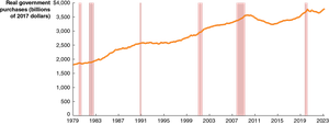
• Government purchases (G): All levels of government spending on goods and services (excludes transfer payments).

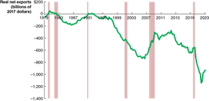
• Net exports (NX): Exports minus imports.

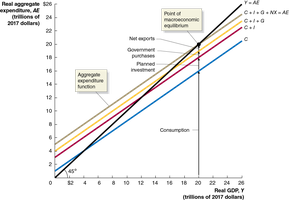
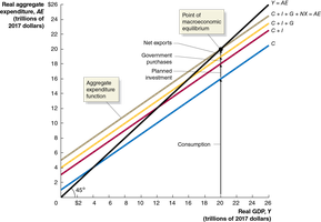
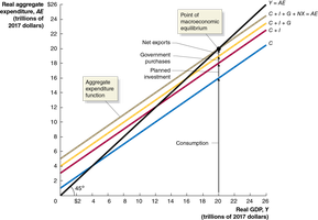
• Aggregate expenditure (AE): The sum of C, I, G, and NX.

Planned vs. Actual Investment

• Planned investment excludes unplanned changes in inventories, while actual investment includes them.

• Macroeconomic equilibrium occurs when planned investment equals actual investment (no unplanned inventory changes).

Determinants of Aggregate Expenditure

Consumption

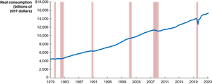
Consumption is the largest component of aggregate expenditure and is influenced by several factors:

• Current disposable income: Higher income leads to higher consumption.

• Household wealth: Net assets increase consumption; a $1,000 increase in wealth typically raises annual consumption by $40–$50.

• Expected future income: Households smooth consumption over time, considering both current and expected income.

• Price level: Higher prices reduce real wealth and consumption.

• Interest rate: Higher rates encourage saving and reduce consumption, especially of durable goods.

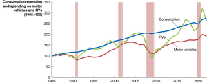
Volatility of Durable Goods Consumption

• Spending on durable goods is more volatile than overall consumption due to postponable purchases, substitutes, and sensitivity to interest rates.

The Consumption Function and Marginal Propensity to Consume (MPC)

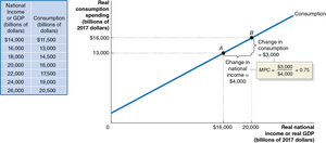
• Consumption function: The relationship between consumption and disposable income.

• Marginal propensity to consume (MPC): The change in consumption from a change in disposable income; it is the slope of the consumption function.

Marginal Propensity to Save (MPS)

• Marginal propensity to save (MPS): The change in saving from a change in disposable income.

• MPC + MPS = 1.

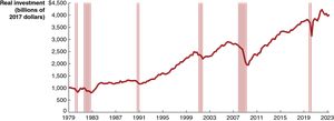
Planned Investment

• Expectations of future profitability: Optimism increases investment; pessimism reduces it.

• Interest rate: Higher rates decrease investment; lower rates increase it.

• Taxes: Higher corporate taxes reduce investment; tax incentives increase it.

• Cash flow: Higher profits (cash flow) enable more investment.

Government Purchases

• Includes all levels of government spending on goods and services (not transfer payments).

• Generally increases over time, with exceptions during certain periods (e.g., post-Cold War, post-2007–2009 recession).

Net Exports

• Determined by the price level, growth rates, and exchange rates relative to other countries.

• U.S. net exports have been negative for decades, typically rising (becoming less negative) during recessions as imports fall.

Graphing Macroeconomic Equilibrium

The 45-Degree Line Diagram

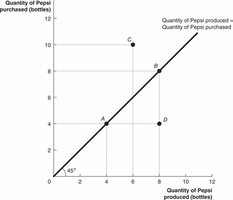
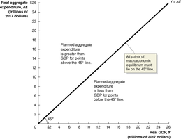
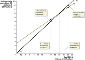
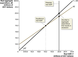
• Equilibrium occurs where aggregate expenditure equals real GDP (on the 45-degree line).

• Points above the line: AE > GDP (inventories fall, production rises).

• Points below the line: AE < GDP (inventories rise, production falls).

The Role of Inventories

• Unplanned inventory changes signal firms to adjust production, moving the economy toward equilibrium.

The Multiplier Effect

Definition and Calculation

• Multiplier effect: A small change in autonomous expenditure leads to a larger change in equilibrium real GDP.

• Multiplier formula: $\text{Multiplier} = \frac{1}{1 - \text{MPC}}$

• Example: If MPC = 0.75, then Multiplier = 4.

Process of the Multiplier

• An initial increase in autonomous expenditure increases GDP, which induces further increases in consumption and GDP, and so on.

• The process continues until the total change in GDP is a multiple of the initial change in expenditure.

Reverse Multiplier

• The multiplier works in reverse: a decrease in autonomous expenditure leads to a multiplied decrease in GDP (e.g., during the Great Depression).

Summary of the Multiplier

• The multiplier is always greater than 1.

• The higher the MPC, the larger the multiplier.

• Real-world factors (imports, taxes, inflation) can reduce the actual multiplier below the theoretical value.

The Paradox of Thrift

• Recall the savings identity: savings equals investment

  • This implies that savings were the key to long-term economic growth

  • If people save more, then consumption decrease and hence income increases, so consumption decreases... potentially pushing the economy into recession

• Increased saving can reduce consumption and income in the short run, potentially causing a recession, even though saving is beneficial in the long run.

The Aggregate Demand Curve

Relationship to Aggregate Expenditure

• The aggregate demand (AD) curve shows the inverse relationship between the price level and the quantity of real GDP demanded.

• As the price level rises, aggregate expenditure and real GDP fall; as the price level falls, aggregate expenditure and real GDP rise.

Why the AD Curve Slopes Downward

• Higher price levels reduce real wealth, decreasing consumption.

• Higher U.S. prices reduce exports and increase imports, lowering net exports.

• Higher prices increase the demand for money, raising interest rates and reducing investment.

Appendix: The Algebra of Macroeconomic Equilibrium

Aggregate Expenditure Equations

• Consumption function: $C = a + bY$

• Planned investment: $I = I_0$

• Government purchases: $G = G_0$

• Net exports: $NX = NX_0$

• Equilibrium condition: $Y = C + I + G + NX$

Solving for Equilibrium GDP

• Substitute the first four equations into the equilibrium condition and solve for $Y$:

$Y = a + bY + I_0 + G_0 + NX_0$

$Y - bY = a + I_0 + G_0 + NX_0$

$Y(1 - b) = a + I_0 + G_0 + NX_0$

$Y = \frac{a + I_0 + G_0 + NX_0}{1 - b}$

• This formula shows how equilibrium GDP depends on autonomous expenditures and the marginal propensity to consume.

Summary Table: Key Concepts

Concept	Definition
Aggregate Expenditure (AE)	Total spending in the economy (C + I + G + NX)
Macroeconomic Equilibrium	Occurs when AE = Real GDP
Marginal Propensity to Consume (MPC)	Change in consumption from a change in income
Multiplier	$\frac{1}{1 - \text{MPC}}$
Aggregate Demand Curve	Shows relationship between price level and real GDP demanded