 Back
BackChapter 10 for final exam studying
Study Guide - Smart Notes
 Tailored notes based on your materials, expanded with key definitions, examples, and context.
Expenditure Plans and the Circular Flow
Aggregate Planned Expenditure
The aggregate planned expenditure (AE) is the total amount of spending planned in an economy, including consumption, investment, government purchases, exports, and imports. The formula for aggregate planned expenditure is:
AE = C + I + G + X - IM
C: Planned consumption spending
I: Planned business investment spending
G: Planned government purchases
X: Planned exports
IM: Planned imports
In the circular flow model, aggregate spending equals aggregate income (Y), so:
AE = Y in equilibrium
Income, Spending, Saving, and Taxes
All income in the economy is either spent, saved, or taxed:
Y = C + S + T
Where S is savings and T is net taxes
Rearranging the aggregate expenditure equation gives:
I + G + X = S + T + IM
This shows that injections (I, G, X) must equal leakages (S, T, IM) in equilibrium
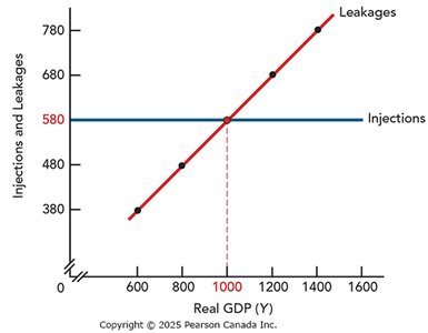
Injections and Leakages
Injections are sources of spending that do not originate with consumers, such as government purchases, business investment, and exports. Leakages are uses of income that remove spending from the circular flow, such as savings, taxes, and imports.
Injections = I + G + X
Leakages = S + T + IM
Equilibrium occurs when injections equal leakages.
The Bathtub Model
The bathtub model is a metaphor for the circular flow of income. If injections exceed leakages, the 'water level' (real GDP) rises. If leakages exceed injections, the water level falls. Prices are assumed fixed, so all adjustments occur through changes in real GDP.
If injections > leakages, real GDP increases
If leakages > injections, real GDP decreases
The Consumption Function and Marginal Propensities
Consumption Function
The consumption function shows the relationship between planned consumption (C) and disposable income (YD):
C = 0.8YD
YD = Y - T, where T is taxes (e.g., T = 100)
So, C = 0.8(Y - 100) = 0.8Y - 80
The marginal propensity to consume (MPC) is the fraction of a change in disposable income that is spent on consumption. In this example, MPC = 0.8.
Savings Function and Marginal Propensity to Save
All disposable income is either spent or saved:
C + S = YD
S = YD - C
Given C = 0.8YD, S = 0.2YD
The marginal propensity to save (MPS) is the fraction of a change in disposable income that is saved. Here, MPS = 0.2.
MPC + MPS = 1
Autonomous and Induced Spending
Autonomous spending is the part of aggregate planned expenditure that does not depend on real GDP (Y). In the simple AE model, investment (I), government spending (G), and exports (X) are assumed fixed:
I = 250
G = 150
X = 180
Induced spending depends on real GDP. For example:
C = 0.8Y - 80
IM = 0.3Y (planned imports depend on income)
The marginal propensity to import (MPIM) is the fraction of a change in income spent on imports (0.3 in this example).
The Aggregate Expenditure Model
Aggregate Expenditure Equation
The aggregate expenditure model combines all components:
AE = C + I + G + X - IM
Given the values above:
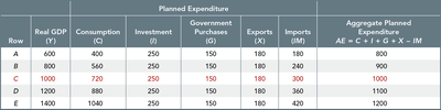
Tabular Example of Planned Expenditure
The following table illustrates how aggregate planned expenditure is calculated for different levels of real GDP:
Row | Real GDP (Y) | Consumption (C) | Investment (I) | Government Purchases (G) | Exports (X) | Imports (IM) | Aggregate Planned Expenditure (AE) |
|---|---|---|---|---|---|---|---|
A | 600 | 400 | 250 | 150 | 180 | 180 | 800 |
B | 800 | 540 | 250 | 150 | 180 | 240 | 1000 |
C | 1000 | 720 | 250 | 150 | 180 | 300 | 1000 |
D | 1200 | 880 | 250 | 150 | 180 | 360 | 1100 |
E | 1400 | 1040 | 250 | 150 | 180 | 420 | 1200 |
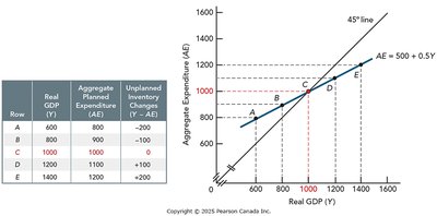
Graphical Representation of Equilibrium
Equilibrium expenditure occurs where aggregate planned expenditure equals real GDP. This is shown where the AE function crosses the 45º line on a graph. At equilibrium:
AE = Y
Using the equation:
Solving:
At this point, unplanned inventory changes are zero, and the economy is in equilibrium.
Row | Real GDP (Y) | Aggregate Planned Expenditure (AE) | Unplanned Inventory Changes (Y - AE) |
|---|---|---|---|
A | 600 | 800 | -200 |
B | 800 | 1000 | -200 |
C | 1000 | 1000 | 0 |
D | 1200 | 1100 | 100 |
E | 1400 | 1200 | 200 |
Injections, Leakages, and Equilibrium
Equilibrium in the aggregate expenditure model is achieved only when injections equal leakages. If real GDP is below equilibrium, injections exceed leakages, causing GDP to rise. If real GDP is above equilibrium, leakages exceed injections, causing GDP to fall. At equilibrium, there is no tendency for GDP to change.
Below equilibrium: AE > Y, GDP rises
Above equilibrium: AE < Y, GDP falls
At equilibrium: AE = Y, GDP stable
Summary Table: Key Formulas
Concept | Formula |
|---|---|
Aggregate Planned Expenditure | |
Consumption Function | |
Imports Function | |
Equilibrium Condition | |
Equilibrium Solution | |
MPC + MPS |
