Aggregate Supply, Aggregate Demand, and Macroeconomic Fluctuations: Study Notes

Aggregate Supply

Long-Run Aggregate Supply (LAS)

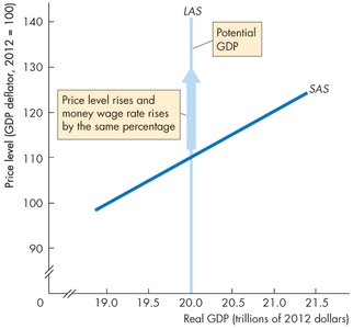
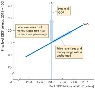
The long-run aggregate supply (LAS) curve shows the relationship between the quantity of real GDP supplied and the price level when real GDP equals potential GDP. In the long run, potential GDP is determined by the economy's resources and technology, and is independent of the price level. The LAS curve is vertical at the level of potential GDP.

• Potential GDP: The maximum sustainable output of an economy, determined by the full-employment quantity of labor, the stock of capital, and technology.

• LAS Curve: Vertical because changes in the price level do not affect potential GDP in the long run.

• Adjustment Mechanism: In the long run, money wages and other input prices adjust to match changes in the price level, keeping real GDP at potential GDP.

Short-Run Aggregate Supply (SAS)

The short-run aggregate supply (SAS) curve shows the relationship between the quantity of real GDP supplied and the price level when money wages and other input prices are held constant. The SAS curve is upward sloping because, in the short run, a higher price level increases firms' profits and induces them to increase production.

• SAS Curve: Upward sloping because input prices are sticky in the short run.

• Short-Run Response: Firms increase output when the price level rises, as long as input prices remain unchanged.

Shifts in Aggregate Supply

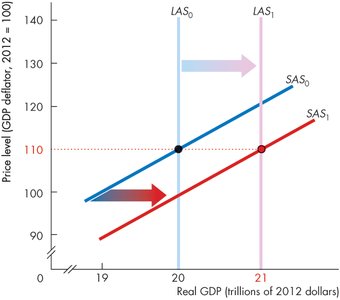
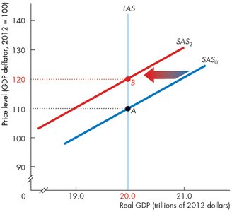
Aggregate supply shifts when factors other than the price level change production plans. These include changes in potential GDP, the money wage rate, and other input prices.

• Increase in Potential GDP: Shifts both LAS and SAS curves rightward.

• Increase in Money Wage Rate: Shifts the SAS curve leftward but does not affect the LAS curve.

• Causes of Potential GDP Change: Changes in the full-employment quantity of labor, capital stock, or technology.

Aggregate Demand

Definition and Components

Aggregate demand (AD) is the total quantity of final goods and services demanded in an economy at different price levels. It is the sum of consumption (C), investment (I), government expenditure (G), and net exports (X – M):

$Y = C + I + G + X - M$

• Consumption (C): Household spending on goods and services.

• Investment (I): Business spending on capital goods.

• Government Expenditure (G): Government purchases of goods and services.

• Net Exports (X – M): Exports minus imports.

Determinants of Aggregate Demand

• Price Level: Affects the purchasing power of money and influences the quantity of real GDP demanded.

• Expectations: About future income, inflation, and profits.

• Fiscal Policy: Changes in taxes, transfer payments, and government spending.

• Monetary Policy: Changes in interest rates and the money supply.

• The World Economy: Changes in foreign income and exchange rates.

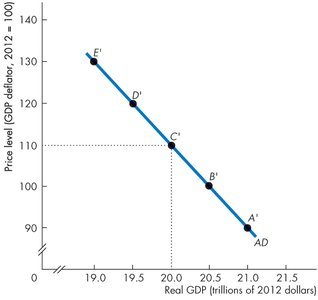
Shape of the Aggregate Demand Curve

The AD curve slopes downward due to the wealth effect and substitution effects:

• Wealth Effect: A higher price level reduces real wealth, leading to less consumption and a lower quantity of real GDP demanded.

• Intertemporal Substitution Effect: Higher price levels raise interest rates, reducing borrowing and spending.

• International Substitution Effect: Higher domestic prices make exports less competitive, reducing net exports.

Shifts in Aggregate Demand

Any change in determinants other than the price level shifts the AD curve. For example:

• Increased Expected Future Income: Increases consumption and shifts AD rightward.

• Expansionary Fiscal Policy: Tax cuts or increased government spending shift AD rightward.

• Expansionary Monetary Policy: Lower interest rates or increased money supply shift AD rightward.

• Growth in Foreign Income: Increases demand for exports, shifting AD rightward.

Macroeconomic Fluctuations

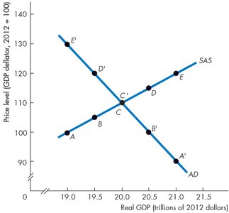
Short-Run Macroeconomic Equilibrium

Short-run equilibrium occurs where the AD and SAS curves intersect. At this point, the quantity of real GDP demanded equals the quantity supplied, but real GDP may be above or below potential GDP.

• Short-Run Equilibrium: Real GDP can be greater than, less than, or equal to potential GDP.

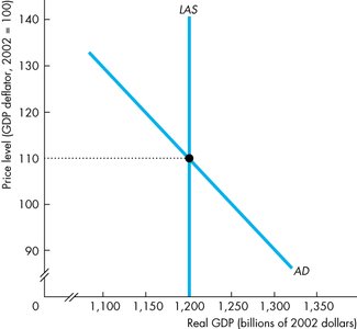
Long-Run Macroeconomic Equilibrium

Long-run equilibrium occurs when real GDP equals potential GDP, i.e., at the intersection of the AD and LAS curves. Over time, adjustments in the money wage rate move the economy toward long-run equilibrium.

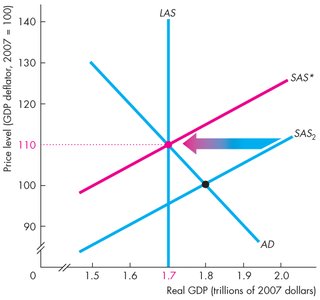
• Adjustment Mechanism: If real GDP is above potential, money wages rise, shifting SAS leftward. If real GDP is below potential, money wages fall, shifting SAS rightward.

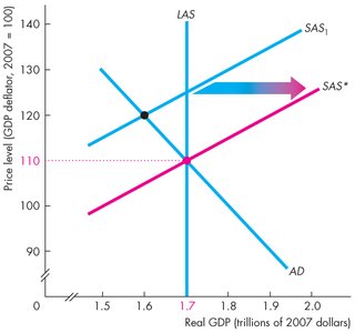
Adjustment to Long-Run Equilibrium

When the economy is not at long-run equilibrium, the money wage rate adjusts over time to restore equilibrium at potential GDP.

• Below Full-Employment Equilibrium: Money wages fall, shifting SAS rightward until real GDP returns to potential.

• Above Full-Employment Equilibrium: Money wages rise, shifting SAS leftward until real GDP returns to potential.

Economic Growth in the AS-AD Model

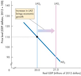
Economic growth is represented by a rightward shift of the LAS curve, reflecting increases in potential GDP due to growth in labor, capital, or technology.

• LAS Shift: Indicates higher potential output for the economy.

Inflation in the AS-AD Model

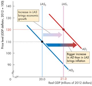
If aggregate demand increases faster than long-run aggregate supply, the result is inflation—a sustained rise in the price level.

• AD Shift: A rightward shift in AD greater than the shift in LAS causes inflation.

The Business Cycle in the AS-AD Model

The business cycle arises from fluctuations in aggregate demand and short-run aggregate supply, with the money wage rate adjusting too slowly to keep real GDP at potential GDP.

• Below Full-Employment Equilibrium: Potential GDP exceeds real GDP (recessionary gap).

• Above Full-Employment Equilibrium: Real GDP exceeds potential GDP (inflationary gap).

• Full-Employment Equilibrium: Real GDP equals potential GDP (no output gap).

Type of Gap	Condition
Inflationary Gap	Potential GDP < Real GDP
No Output Gap	Potential GDP = Real GDP
Recessionary Gap	Potential GDP > Real GDP

Inflation Cycles

Demand-Pull Inflation

Demand-pull inflation occurs when aggregate demand increases, causing the price level to rise. This can be triggered by factors such as lower interest rates, increased government spending, or higher expected future income.

• Initial Effect: AD shifts right, creating an inflationary gap.

• Adjustment: SAS shifts left as money wages rise, returning real GDP to potential but at a higher price level.

• Ongoing Process: Sustained by continuous increases in aggregate demand, often due to ongoing increases in the money supply.

Cost-Push Inflation

Cost-push inflation starts with an increase in production costs, such as higher money wage rates or increased prices of raw materials (e.g., oil). This shifts the SAS curve leftward, reducing real GDP and raising the price level (stagflation).

• Initial Effect: SAS shifts left, creating a recessionary gap.

• Policy Response: If the central bank increases aggregate demand to counter unemployment, the price level rises further.

• Stagflation: Combination of rising prices and falling real GDP.

Expected Inflation

When increases in aggregate demand are anticipated, money wages rise in line with expected price increases, keeping real GDP at potential GDP but at a higher price level. The process repeats as long as expectations are accurate.

Inflation and the Business Cycle

If aggregate demand grows faster than expected, real GDP temporarily exceeds potential GDP, leading to higher-than-expected inflation (demand-pull). If aggregate demand grows more slowly than expected, real GDP falls below potential GDP, and inflation slows (cost-push).

Summary Table: Types of Inflation

Type	Cause	Effect
Demand-Pull	Increase in AD	Higher price level, temporary rise in real GDP
Cost-Push	Increase in costs (wages, raw materials)	Higher price level, lower real GDP (stagflation)
Expected	Anticipated AD increase	Higher price level, real GDP at potential

Additional info: The above notes integrate textbook-level explanations, equations, and tables to provide a comprehensive, exam-ready summary of aggregate supply, aggregate demand, macroeconomic equilibrium, and inflation cycles, as covered in a college-level macroeconomics course.