 Back
BackApplications and Extensions of Demand and Supply: Price Controls, Taxes, and Subsidies
Study Guide - Smart Notes
 Tailored notes based on your materials, expanded with key definitions, examples, and context.
Demand and Supply: Applications and Extensions
The Link Between Resource and Product Markets
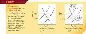
Resource and product markets are fundamentally interconnected in the macroeconomy. Businesses demand resources (such as labor) to produce goods and services, while households supply these resources in exchange for income. Changes in resource markets can directly impact product markets and vice versa.
Resource Market: Firms demand resources (e.g., labor), and households supply them.
Product Market: Firms supply goods and services, and households demand them.
Example: A decrease in the supply of young workers increases wages for restaurant staff, raising restaurant costs and leading to higher meal prices.
Resource Prices and Product Markets
Changes in resource prices, such as wages, affect the cost structure of firms and thus the supply of goods in product markets. Higher resource prices typically reduce supply, leading to higher equilibrium prices for final goods.
The Economics of Price Controls
Price Ceilings
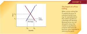
A price ceiling is a legal maximum price that can be charged for a good or service. When set below the market equilibrium, it leads to shortages and non-price rationing mechanisms.
Direct Effect: Shortage, as quantity demanded exceeds quantity supplied.
Indirect Effects: Quality deterioration, waiting lines, and allocation by non-price factors.
Example: Rent control in housing markets.
Price Floors
A price floor is a legal minimum price for a good or service. When set above equilibrium, it results in surpluses and inefficiencies.
Direct Effect: Surplus, as quantity supplied exceeds quantity demanded.
Indirect Effects: Non-price allocation mechanisms, such as favoritism or waste.
Example: Minimum wage laws in labor markets.

Minimum Wage as a Price Floor
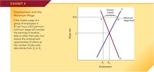
The minimum wage is a classic example of a price floor in the labor market. When set above the equilibrium wage, it increases wages for some but reduces employment opportunities for others, especially low-skilled workers.
Direct Effect: Reduced employment for low-skilled labor.
Indirect Effects: Reduced non-wage benefits, less on-the-job training, and potential increase in school dropouts.
Graphical Example: Employment falls from E0 to E1 as minimum wage rises above equilibrium.
The Impact of Taxes
Tax Incidence
Tax incidence refers to the actual distribution of the tax burden between buyers and sellers, which may differ from the statutory assignment. The burden depends on the relative elasticities of demand and supply.
Statutory Incidence: Who is legally responsible for paying the tax.
Economic Incidence: Who actually bears the cost, determined by market forces.
Impact of a Tax Imposed on Sellers
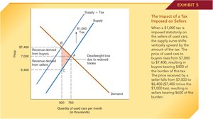
When a tax is imposed on sellers, the supply curve shifts upward by the amount of the tax. The new equilibrium price rises, but not by the full amount of the tax. Both buyers and sellers share the burden.
Example: A $1,000 tax on used car sellers raises the price from $7,000 to $7,400. Sellers net $6,400 after tax, buyers pay $7,400. The burden is split: buyers pay $400, sellers $600.
Deadweight Loss: The reduction in total surplus due to the tax.
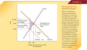
Impact of a Tax Imposed on Buyers
When a tax is imposed on buyers, the demand curve shifts downward by the amount of the tax. The new equilibrium price falls, but buyers pay the tax on top of this price. The burden is again shared.
Example: A $1,000 tax on buyers results in a net price of $7,400 for buyers, $6,400 for sellers. The burden is the same as when imposed on sellers.
Key Point: The incidence is the same regardless of statutory assignment.
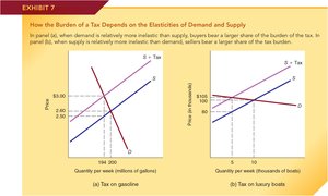
Elasticity and the Burden of the Tax
The division of the tax burden depends on the relative elasticities of demand and supply. The side of the market that is more inelastic bears a greater share of the tax burden.
Inelastic Demand: Buyers bear more of the tax (e.g., gasoline).
Inelastic Supply: Sellers bear more of the tax (e.g., luxury boats).
Tax Rates, Tax Revenues, and the Laffer Curve
Average and Marginal Tax Rates
Average tax rate is the total tax paid divided by total income. Marginal tax rate is the tax rate on the next dollar of income. These concepts are crucial for understanding tax policy and its effects on behavior.
Formula for Average Tax Rate:
Formula for Marginal Tax Rate:
Example: If tax liability increases from \frac{22}{100} = 22\%$.

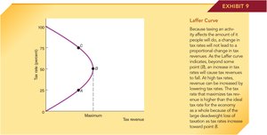
The Laffer Curve
The Laffer Curve illustrates the relationship between tax rates and tax revenues. At both 0% and 100% tax rates, revenue is zero. There is a tax rate between these extremes that maximizes revenue, but higher rates beyond this point reduce the tax base and total revenue.
Key Point: Increasing tax rates beyond a certain point can decrease total tax revenue due to reduced economic activity.
The Impact of a Subsidy
Impact of a Subsidy Granted to Buyers
When the government grants a subsidy to buyers, the demand curve shifts upward by the amount of the subsidy. This increases the equilibrium price and quantity, benefiting both buyers (who pay less net of subsidy) and sellers (who receive a higher price).
Example: A $4,000 tuition subsidy raises the gross price from $10,000 to $12,000, but subsidized students pay only $8,000. Both students and colleges benefit.
Distribution of Benefits: The more inelastic the supply, the greater the benefit to suppliers.

Real World Subsidy Programs
Subsidy programs are widespread and often benefit suppliers as much as, or more than, the intended recipients. When only some groups are subsidized, non-subsidized groups may face higher prices.
Example: College tuition subsidies benefit both students and colleges, but may raise prices for non-subsidized students.
