Chapter 16: Fiscal Policy – Macroeconomics Study Notes

Fiscal Policy: Concepts and Applications

What Is Fiscal Policy?

Fiscal policy refers to the use of government spending, transfer payments, and taxation to influence macroeconomic outcomes such as real GDP, unemployment, and inflation. It is primarily conducted by the federal government, with state and local policies generally not aimed at national objectives.

• Before the Great Depression, state and local governments did most of the spending, but today the federal government is responsible for about two-thirds to three-quarters of all government spending.

• Automatic stabilizers: Government spending and taxes that automatically increase or decrease with the business cycle (e.g., unemployment insurance).

• Discretionary fiscal policy: Deliberate changes in government spending or taxes to achieve macroeconomic goals.

• Example: During recessions, unemployment insurance payments rise automatically, helping to stabilize income and demand.

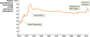
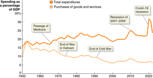
Federal Government Expenditures and Revenue

The composition of federal government spending and revenue sources is crucial for understanding fiscal policy's scope and limitations.

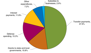
The federal government spends money in three main ways:

1. Government purchases – Money spent on goods and services, such as:

   • National defense (military)

   • Salaries for FBI agents and other federal employees

   • Operating national parks

   • Funding scientific research

2. Grants to state and local governments – Money given to states and cities to help pay for programs like:

   • Education

   • Crime prevention

   • Public transportation

   • Other local services

3. Interest on the federal debt – Money the government pays to people and organizations that have loaned it money by buying U.S. Treasury bonds.

• Expenditures: Include defense, salaries, national parks, scientific research, transfer payments (Social Security, Medicare), grants to states, and interest on debt.

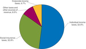
• Revenue: Primarily from individual income taxes and payroll taxes, with smaller shares from corporate taxes, excise taxes, tariffs, and other fees.

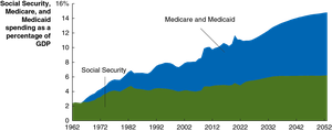
Social Security and Medicare: Fiscal Challenges

Programs like Social Security and Medicare have reduced poverty among the elderly but face long-term funding challenges due to demographic changes and rising healthcare costs.

• Through 2092, the budget shortfall for these programs is estimated to be enormous:

  almost $16.8 trillion (in present value terms).

• Potential solutions: Increasing taxes, reducing benefits, raising eligibility ages (SSI age already increasing from 65 to 67), and controlling medical costs.

The Effects of Fiscal Policy on Real GDP and the Price Level

Fiscal Policy and Aggregate Demand

Fiscal policy affects aggregate demand (AD) through changes in government purchases and taxes:

Congress and the president carry out fiscal policy through:

• Changes in government purchases

• Changes in taxes

AD = C +I + G + NX

• G directly affects AD

  • A change in taxes changes income; this in turn affects consumption, and so it has an indirect effect on aggregate demand

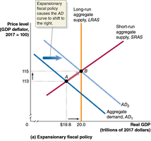
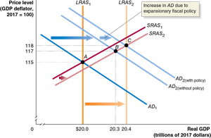
• Expansionary fiscal policy: Increases government purchases or decreases taxes to boost AD and reduce unemployment when real GDP is below potential (this occurs when there's a recession, meaning real GDP is below Potential GDP. The gov. can enact this to restore long-run equilibrium decreasing unemployment )

  • One cost: high inflation

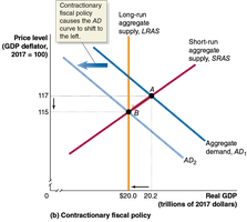
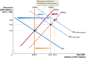
• Contractionary fiscal policy: Decreases government purchases or increases taxes to reduce AD and control inflation when real GDP exceeds potential. (when inflation is to high the gov. will enact this, meaning Real GDP is above the Potential GDP, decreasing inflation (the aggregate price level))

Fiscal Policy During Economic Shocks

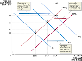
During events like the Covid-19 pandemic, both aggregate supply and demand can shift. Expansionary fiscal policy can help restore GDP but may also contribute to inflation.

Fiscal Policy in the Dynamic Aggregate Demand and Aggregate Supply Model

The dynamic AD-AS model incorporates changes in potential GDP and the price level over time, providing a more realistic framework for analyzing fiscal policy.

• Our model of fiscal policy so far is static: it assumes long-run potential GDP does not change and that the price level is constant.

• Expansionary policy: Used when projected AD growth is insufficient

• for full employment, raising both real GDP and the price level.

• Contractionary policy: Used when projected AD growth is excessive, reducing inflationary pressures.

The Government Purchases, Tax, and Transfer Payment Multipliers

The Multiplier Effect

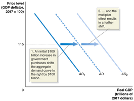
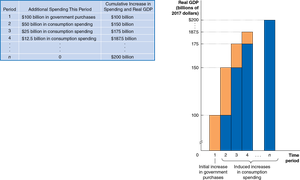
The multiplier effect describes how an initial change in autonomous expenditure (such as government purchases) leads to a larger change in real GDP due to induced increases in consumption.

• Government purchases multiplier: Measures the total change in GDP from a change in government spending.

• Tax multiplier: Measures the total change in GDP from a change in taxes (negative value; smaller in absolute terms than the purchases multiplier).

• Transfer payments multiplier: Positive effect on GDP as increased transfers raise disposable income and consumption.

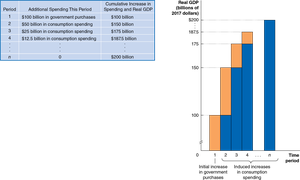
Formulas for Multipliers (loot at notes)

• There's an inverse relationship between taxes and equilibrium real GDP

Multiplier	Formula	Significance
Government Purchases Multiplier	$\frac{1}{1 - MPC}$	Measures total GDP change from government spending
Tax Multiplier	$-\frac{MPC}{1 - MPC}$	Measures total GDP change from tax changes
Balanced Budget Multiplier	1	GDP change when spending and taxes rise equally

Example: If MPC = 0.75, the government purchases multiplier is 4, and the tax multiplier is -3.

The Effect of Changes in the Tax Rate

• The tax multiplier applies to changes in the amount of taxes, without changes in tax rates.

Example: In 2009 and 2010, the federal government enacted the Making Work Pay Tax Credit: a $400 reduction in taxes for working individuals ($800 for households).

Decreases in tax rates have a slightly different effect:

1. Increasing the disposable income of households, leading them to increase their consumption spending

2. Increasing the size of the multiplier effect, since more of any increase in income becomes disposable income

Multiplier and Aggregate Supply

• An increase in aggregate demand will not only raise real GDP; it will also raise the price level because the short-run aggregate supply curve is upward sloping.

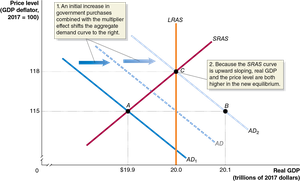
The Multipliers Work in Both Directions

• An increase in government purchases and a cut in taxes have a positive multiplier effect.

• A decrease in government purchases, and an increase in taxes have a negative multiplier effect.

  Example: A reduction in government spending on defense initially affects defense contractors, but then it would spread to suppliers to and employees of those contractors and then to other firms and workers.

Limits to Using Fiscal Policy to Stabilize the Economy

• Fiscal policy is often less effective than monetary policy for stabilizing the economy.

• Timing delays reduce fiscal policy's effectiveness:

  • Legislative delay: Congress takes time to approve policies.

  • Implementation delay: Approved spending projects can take months or years to start.

• Crowding out: Increased government spending can reduce private spending (by households and businesses), limiting the overall impact of fiscal policy.

Recession of 2007-2009 was 18 months

Average for postwar recessions was 10.4 months

Deficits, Surpluses, and Federal Government Debt

Definitions and Trends

• Budget deficit: Government expenditures exceed tax revenue.

• Budget surplus: Government expenditures are less than tax revenue.

• Federal debt: The total value of outstanding Treasury securities.

The Effect of Crowding Out in the Short Run

• Increase in government spending → decreases the supply of loanable funds.

• Interest rates rise as a result.

• Higher interest rates reduce:0

  • Consumption

  • Investment

  • Net exports

• Crowding out: The increase in government spending is partially offset because private spending falls.

Crowding Out in the Long Run

• In the long run, government spending does not increase real GDP because the economy returns to potential GDP.

• Crowding out fully offsets the increase in government spending by reducing consumption, investment, and net exports.

• The main long-run effect is a larger government sector in the economy.

• Short-run increases in GDP may still be beneficial, even though the long-run effect disappears.

American Recovery and Reinvestment Act of 2009

• American Recovery and Reinvestment Act (2009): An $840 billion stimulus package, the largest U.S. fiscal policy at the time.

• About two-thirds of the package was increased government spending, with effects lasting through 2013.

• The remaining one-third consisted of tax cuts and tax credits.

• Tax cuts had quicker effects, mostly occurring between 2009 and 2011.

  • Isolating the effects of the stimulus package is very difficult; economists still differ in their views about how effective the stimulus package was.

  • The CBO’s conclusion: the stimulus package reduced the severity of the

    recession but did not come close to bringing the economy back to full

    employment.

• Gov purchase multipliers and tax multipliers are difficult to measure

Deficits, Surpluses and Federal Government Debt

• A budget deficit is the situation in which the government’s expenditures are greater than its tax revenue.

• A budget surplus is the situation in which the government’s expenditures are less than its tax revenue

Federal Budget Balance = Tax Revenue (T) - Gov. Expenditure (G)

• T < G, budget deficit

• T> G, budget surplus

• Most developing countries run a deficit

Automatic Stabilizers and the Cyclically Adjusted Budget

Automatic stabilizers help limit the severity of recessions by increasing deficits during downturns. The cyclically adjusted budget deficit/surplus estimates what the budget would be if GDP were at potential.

Key Concepts

• Budget deficits increase during recessions because tax revenue falls and automatic stabilizers (like unemployment benefits and food stamps) increase spending.

• Automatic stabilizers help reduce the severity of recessions by supporting household income and spending.

• Cyclically adjusted budget deficit/surplus: The budget balance if the economy were at potential GDP, removing the effects of the business cycle.

• In 2009, the federal deficit was 9.3% of GDP:

  • 7.6% was due to government spending and tax policies.

  • 1.7% was due to automatic stabilizers during the recession.

• Most economists believe the budget should be balanced at potential GDP, but not during a recession, since cutting spending or raising taxes would worsen the downturn.

• Some economists argue that running deficits is acceptable to finance long-term investments, just as households and businesses borrow for major investments.

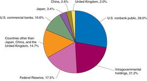
Ownership of the National Debt

• About 40% is held by the government itself (trust funds, Federal Reserve).

• Another 40% is held by U.S. banks and investors.

• The remaining 23% is held by foreign entities.

Is Government Debt a Problem?

While current debt levels are manageable, a rising debt-to-GDP ratio can crowd out investment and hinder long-term growth. Debt used for productive investment (infrastructure, education) is less problematic.

Long-Run Fiscal Policy and Economic Growth

Supply-Side Economics

Long-run fiscal policy aims to increase potential GDP by improving incentives to work, save, invest, and innovate, often through tax policy changes.

• Tax wedge: The difference between pre-tax and post-tax returns to economic activity; larger wedges reduce incentives and GDP.

• Marginal tax rates: Affect labor supply, investment, and saving decisions.

• Tax simplification: Reduces compliance costs and increases efficiency.

Growth Accounting

• Real GDP = hours worked x (real GDP/hours worked)

or in growth terms:

• Growth rate of real GDP = Growth rate of hours worked + Growth rate of labor productivity

Appendix: A Closer Look at the Multiplier

Equilibrium GDP Model

• Consumption function: $C = \overline{C} + MPC \times (Y - T)$

• Planned investment: $I = \overline{I}$

• Government purchases: $G = \overline{G}$

• Tax function: $T = \overline{T}$

• Equilibrium: $Y = C + I + G$

Multiplier with Tax Rates and Open Economy

• With a tax rate $t$, disposable income is $Y - tY$.

• With imports, equilibrium: $Y = C + I + G + X - M$

• Multiplier decreases as the marginal propensity to import (MPI) increases.

Example: If $MPC = 0.75$, $t = 0.2$, $MPI = 0.1$, the multiplier is smaller than in a closed economy.