Chapter 6: The Simplest Short-Run Macro Model – Consumption, Investment, Aggregate Expenditure, and Equilibrium

Desired Consumption Expenditure

Autonomous vs. Induced Expenditures

Expenditures in macroeconomics are classified based on their dependence on national income (Y):

• Autonomous expenditures: Do not depend on national income. Examples include certain government spending or investment decisions made independently of current income.

• Induced expenditures: Depend directly on national income. As income rises, these expenditures increase.

Disposable Income and Consumption Function

Disposable income (YD) is the income available to households after taxes:

• Formula: $Y_D = Y - T$

• Where T is taxes.

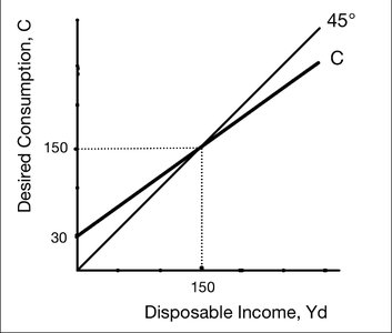
The consumption function models desired consumption as a linear function of disposable income:

• General form: $C = a + bY_D$

• a: Autonomous consumption (consumption when YD = 0)

• b: Marginal propensity to consume (MPC)

Example: $C = 30 + 0.8Y_D$

Marginal Propensity to Consume (MPC)

The MPC is the proportion of additional disposable income that consumers wish to spend:

• Formula: $MPC = \frac{\Delta C}{\Delta Y_D}$

• It is the slope of the consumption function.

Movements and Shifts in the Consumption Function

• Movement along the function: Caused by changes in disposable income.

• Shifts of the function: Caused by changes in wealth, interest rates, or expectations.

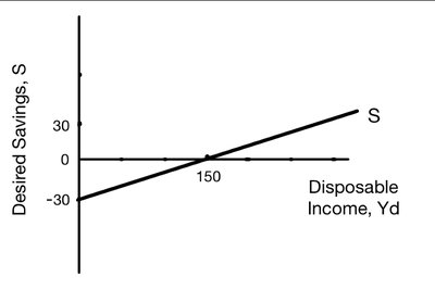
Savings Function

Disposable income not spent is savings:

• Formula: $S = Y_D - C$

• Marginal propensity to save (MPS): $MPS = \frac{\Delta S}{\Delta Y_D}$

Desired Investment Expenditure

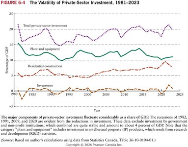
Autonomous Nature and Volatility

Investment is typically considered autonomous, meaning it does not depend on current national income. It is the most volatile component of GDP, strongly associated with short-run economic fluctuations.

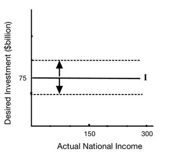
Investment Function

The investment function is usually modeled as a horizontal line, indicating independence from national income:

• Formula: $I = I_0$ (where $I_0$ is autonomous investment)

Shifts in the investment function occur due to:

• Changes in the real interest rate (opportunity cost of investment)

• Changes in the level of sales (inventory and capacity considerations)

• Business confidence (forward-looking expectations)

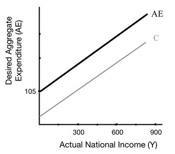
The Aggregate Expenditure Function

Definition and Assumptions

The aggregate expenditure (AE) function relates desired AE to actual national income (Y). In the simplest model:

• No trade: $X = 0$, $IM = 0$

• No government: $G = 0$, $Tax = 0$

• Constant price level

Formula: $AE = C + I$

Example: $C = 30 + 0.8Y$, $I = 75$

Marginal Propensity to Spend (z)

The marginal propensity to spend (z) is the extra desired AE induced by an additional $1 of national income:

• Formula: $z = \frac{dAE}{dY}$

• In this simple model, $z = MPC$

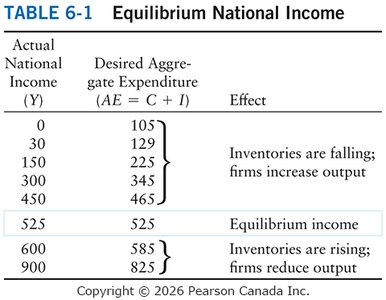
Equilibrium National Income

Definition and Inventory Adjustments

Equilibrium national income is the level where desired aggregate expenditure equals actual national income:

• Condition: $AE = Y$

• If $AE > Y$: Inventories decrease, firms increase output

• If $AE < Y$: Inventories accumulate, firms decrease output

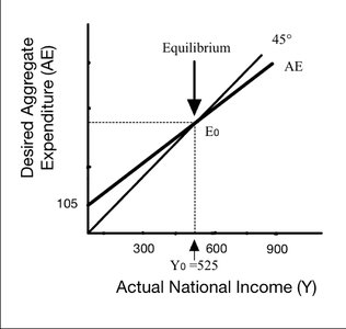
Solving for Equilibrium

Example: $AE = 105 + 0.8Y$

• Equilibrium: $Y_0 = 525$

Actual National Income (Y)	Desired Aggregate Expenditure (AE = C + I)	Effect
0	105	Inventories are falling; firms increase output
30	129	Inventories are falling; firms increase output
150	225	Inventories are falling; firms increase output
300	345	Inventories are falling; firms increase output
450	465	Inventories are falling; firms increase output
525	525	Equilibrium income
600	585	Inventories are rising; firms reduce output
900	825	Inventories are rising; firms reduce output

The Simple Multiplier

Definition and Calculation

The simple multiplier (SM) measures the change in equilibrium national income resulting from a change in desired autonomous expenditure:

• Formula: $SM = \frac{1}{1-z}$

• Where $z$ is the marginal propensity to spend

• Change in income: $\Delta Y = SM \times \Delta A$

The larger the value of $z$, the steeper the AE curve and the larger the multiplier effect.

Example Calculation

• Suppose $C = 30 + 0.75Y$, $I = 40$

• If $I$ increases by 10, the change in equilibrium income is $\Delta Y = SM \times 10$

Additional info: The multiplier effect is central to understanding how changes in autonomous spending (such as government investment or exports) can have amplified effects on national income.