Consumption-Savings Decision in Macroeconomics

Consumption-Savings Decision

Introduction

The consumption-savings decision is a fundamental topic in macroeconomics, focusing on how households allocate their income between current consumption and saving for future consumption. This decision is influenced by factors such as income, interest rates, and fiscal policy, and is central to understanding aggregate demand and investment in the economy.

Key Definitions

• Desired Consumption (Cd): The aggregate quantity of goods and services households wish to consume, given their income and other factors.

• Desired Saving (Sd): The level of national saving when aggregate consumption equals desired consumption. In a closed economy, Sd = Sdp + Sg = Y − Cd − G, where Sdp is desired private saving.

• Consumption-Smoothing Motive: The desire to maintain a relatively stable pattern of consumption over time, often leading to saving during periods of high income and borrowing during periods of low income.

Two-Period Model of Consumption and Saving

To analyze the consumption-savings decision, economists often use a simple two-period model, representing 'today' and 'the future.' Households choose how much to consume in each period, considering their preferences and budget constraints.

• Perfect Capital Markets: No borrowing constraints; the interest rate on savings equals the interest rate on borrowing.

• Indifference Curves: Represent combinations of current (C1) and future (C2) consumption that yield the same utility level.

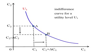
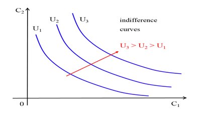
Indifference Curves

Indifference curves illustrate the trade-off between current and future consumption. The slope of the curve at any point shows how much future consumption a consumer is willing to sacrifice for an additional unit of current consumption, keeping utility constant.

• Negatively Sloped: To maintain the same utility, an increase in C1 requires a decrease in C2.

• Higher Curves: Represent higher utility levels.

Budget Constraints

Households face budget constraints in both periods:

• Today: C1 + Sp = V + Y1, where V is initial financial assets.

• Future: C2 = (1 + r)Sp + Y2, where r is the real interest rate.

Combining these yields the intertemporal budget constraint:

$C_1 + \frac{C_2}{1 + r} = V + Y_1 + \frac{Y_2}{1 + r} \equiv W$

• W: Represents total wealth, including initial assets and the present value of income.

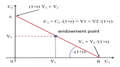
Relative Price and Maximum Consumption

• Relative Price: (1 + r) is the relative price of current consumption to future consumption.

• Maximum Current Consumption: $C_{1,\text{max}} = Y_1 + \frac{Y_2}{1 + r}$

• Maximum Future Consumption: $C_{2,\text{max}} = (1 + r)Y_1 + Y_2$

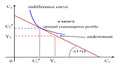
Optimal Consumption Choices

Households choose their optimal consumption profile by maximizing utility subject to their budget constraint. The optimal choice depends on whether the household is a saver or a borrower.

Saver's Optimal Choice

• Savers allocate more to future consumption, resulting in positive savings.

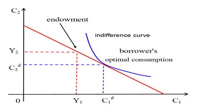
Borrower's Optimal Choice

• Borrowers allocate more to current consumption, resulting in negative savings (borrowing).

Effects of Changes in Income

Increase in Current Income (Y1)

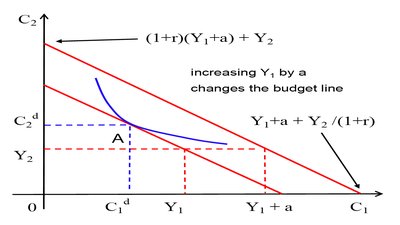
An increase in current income shifts the budget constraint upward, allowing for higher consumption in both periods if consumption is a normal good.

• Parallel Shift: The slope remains unchanged.

• Consumption Increases: Both C1 and C2 rise, as part of the increase is saved for future consumption.

Responses to Higher Y1

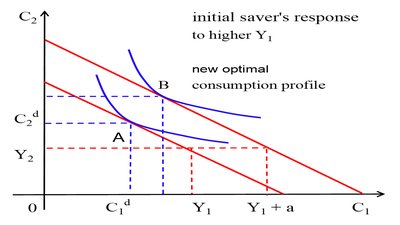
• Saver: Increases both current and future consumption, with new optimal consumption profile.

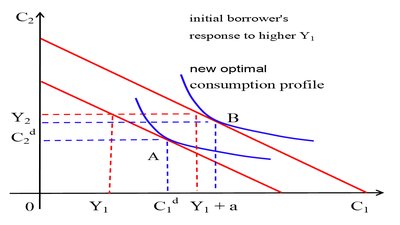
• Borrower: Also increases both current and future consumption, but the effect may differ in magnitude.

Marginal Propensity to Consume (MPC)

The MPC measures the fraction of additional current income that is consumed in the current period:

$\text{MPC} = \frac{\Delta C_1}{\Delta Y_1}$

• MPC < 1: Typically, part of the income increase is saved.

• Implication: An increase in Y1 increases savings.

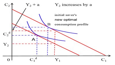
Increase in Future Income (Y2)

An increase in future income shifts the budget constraint, allowing for higher current consumption due to consumption smoothing. Private saving falls, as current income is unchanged.

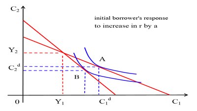
Effects of Changes in the Real Interest Rate (r)

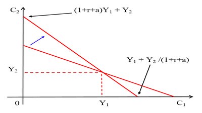
Budget Constraint Rotation

An increase in r rotates the budget constraint clockwise, changing the relative price of current to future consumption.

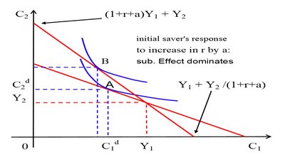
Substitution and Income Effects

• Substitution Effect: Higher r makes future consumption cheaper relative to current consumption, leading consumers to substitute away from current consumption (C1 falls, Sp rises).

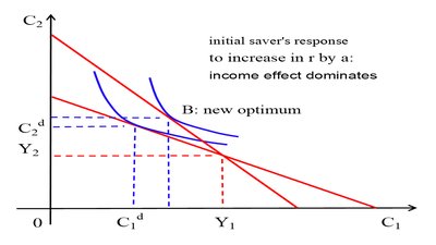
• Income Effect: Depends on whether the consumer is a saver or borrower:

  • Saver (Sp > 0): Higher r increases future income, allowing for higher consumption in both periods.

  • Borrower (Sp < 0): Higher r increases debt burden, reducing consumption in both periods.

Summary Table: Effects of r on Consumption and Saving

	Saver	Borrower
Substitution Effect	Cd1 ↓, Sdp ↑	Cd1 ↓, Sdp ↑
Income Effect	Cd1 ↑, Sdp ↓	Cd1 ↓, Sdp ↑
Overall	Ambiguous	Cd1 ↓, Sdp ↑

Empirical Evidence

• Empirical studies suggest that an increase in r generally reduces current consumption and increases saving, but the effect is not very strong.

Conclusion

The consumption-savings decision is shaped by income, interest rates, and preferences for consumption smoothing. Understanding these dynamics is crucial for analyzing macroeconomic policy and household behavior.