Expenditure Multipliers and Aggregate Expenditure in the Keynesian Model

Expenditure Plans, Marginal Propensities, and the Keynesian Model

Introduction to the Keynesian Model

The Keynesian model analyzes the economy in the very short run, assuming that prices are fixed. In this framework, aggregate demand determines real GDP, and the price level remains constant. The model focuses on how expenditure plans by households, firms, and the government interact to determine output and income.

Aggregate Expenditure and Its Components

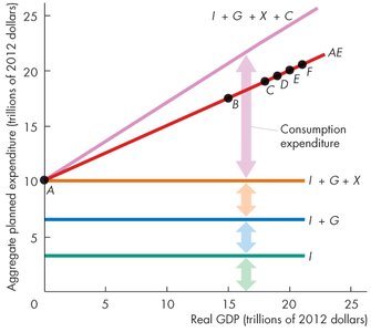
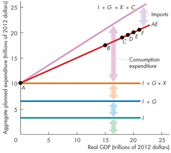
• Aggregate Expenditure (AE): The total planned spending in the economy, given by the equation: $Y = C + I + G + X - M$ where Y is real GDP, C is consumption, I is investment, G is government expenditure, X is exports, and M is imports.

• Two-way Link: An increase in real GDP raises aggregate expenditure, and an increase in aggregate expenditure raises real GDP.

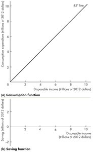
Consumption and Saving Functions

Disposable income (YD) is the income available to households after taxes, defined as:

• $YD = Y - T$

• Disposable income is either consumed (C) or saved (S): $YD = C + S$

The consumption function shows the relationship between consumption and disposable income, while the saving function shows the relationship between saving and disposable income.

Marginal Propensity to Consume (MPC) and Save (MPS)

• MPC: The fraction of a change in disposable income spent on consumption. $MPC = \frac{\Delta C}{\Delta YD}$ Example: If disposable income increases by $2 trillion and consumption increases by $1.5 trillion, then$ MPC = 0.75 $.

• MPS: The fraction of a change in disposable income that is saved. $MPS = \frac{\Delta S}{\Delta YD}$ Example: If disposable income increases by $2 trillion and saving increases by $0.5 trillion, then$ MPS = 0.25 $.

• Relationship: $MPC + MPS = 1$

Marginal Propensity to Import

• The marginal propensity to import is the fraction of an increase in real GDP spent on imports. Example: If an $800 billion increase in real GDP increases imports by $200 billion, the marginal propensity to import is 0.25.

Real GDP with Fixed Prices and Aggregate Expenditure

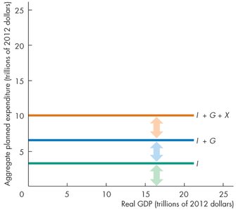
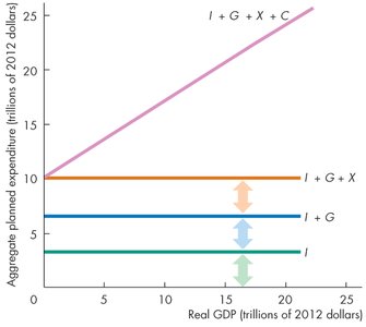
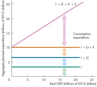
Induced and Autonomous Expenditure

• Induced Expenditure: Consumption expenditure minus imports, which varies with real GDP.

• Autonomous Expenditure: The sum of investment, government expenditure, and exports, which does not vary with GDP. Consumption and imports can also have autonomous components.

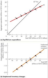
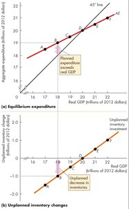
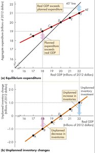
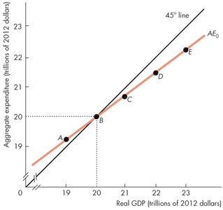
Equilibrium Expenditure

• Actual aggregate expenditure always equals real GDP.

• Planned aggregate expenditure may differ from actual expenditure due to unplanned inventory changes.

• Equilibrium expenditure occurs when planned aggregate expenditure equals real GDP—graphically, where the AE curve crosses the 45° line.

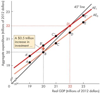
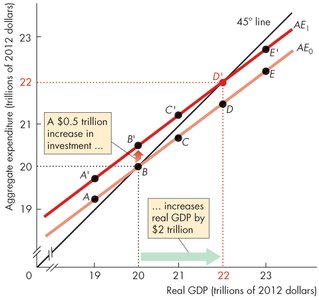
The Expenditure Multiplier

Definition and Process

The multiplier measures how much a change in autonomous expenditure is magnified to determine the change in equilibrium expenditure and real GDP.

• An increase in autonomous expenditure (e.g., investment) increases aggregate expenditure and real GDP.

• This increase leads to higher induced expenditure, causing further increases in aggregate expenditure and real GDP.

• Thus, real GDP increases by more than the initial increase in autonomous expenditure.

Why Is the Multiplier Greater Than 1?

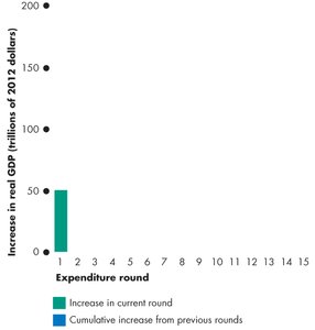
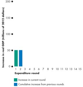
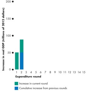
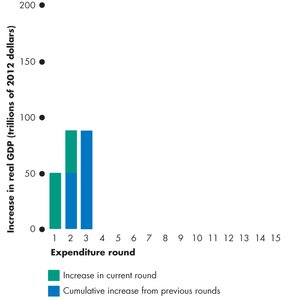
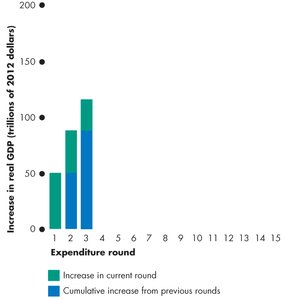
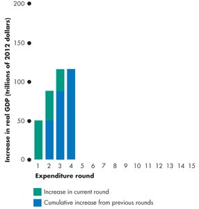
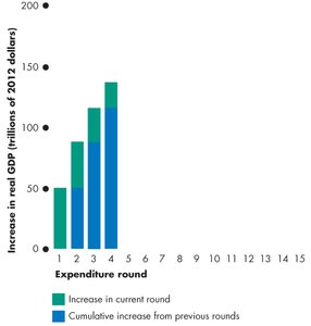
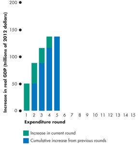
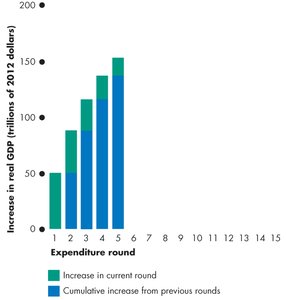
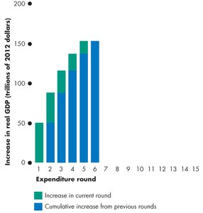
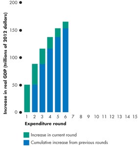
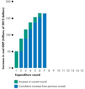
• Each round of increased income leads to further consumption, which induces further increases in aggregate expenditure.

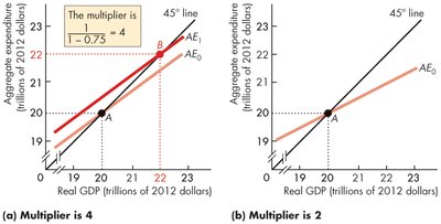
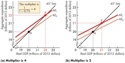
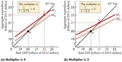
Calculating the Multiplier

• The size of the multiplier is: $Multiplier = \frac{\Delta Y}{\Delta A}$ where $\Delta Y$ is the change in equilibrium real GDP and $\Delta A$ is the change in autonomous expenditure.

• With no taxes or imports: $Multiplier = \frac{1}{1 - MPC}$ Since $1 - MPC = MPS$, $Multiplier = \frac{1}{MPS}$

• With taxes and imports, the multiplier is smaller because these leakages reduce the induced expenditure at each round.

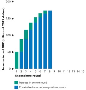
The Multiplier Process

The multiplier process shows how an initial increase in autonomous expenditure leads to successive rounds of increased income and spending, each smaller than the last, until equilibrium is reached.

Linking the Multiplier to the Aggregate Supply-Aggregate Demand (AS-AD) Model

Adjusting Quantities and Prices

• In reality, firms do not keep prices fixed for long. Unplanned changes in inventories lead firms to adjust both production and prices.

• The AS-AD model explains the simultaneous determination of real GDP and the price level, linking the multiplier process to price adjustments.

Aggregate Expenditure and Aggregate Demand Curves

• The aggregate expenditure curve shows the relationship between planned expenditure and real GDP at a fixed price level.

• The aggregate demand curve shows the relationship between the quantity of real GDP demanded and the price level.

• Changes in the price level shift the AE curve and cause movements along the AD curve.

Short-Run and Long-Run Effects

• In the short run, an increase in autonomous expenditure shifts the AE and AD curves, raising real GDP and the price level.

• As the price level rises, the AE curve shifts downward, and equilibrium expenditure decreases.

• In the long run, factor prices adjust, and the multiplier effect on real GDP disappears (the long-run multiplier is zero).

Summary Table: Key Marginal Propensities and the Multiplier

Concept	Definition	Formula
Marginal Propensity to Consume (MPC)	Fraction of additional income spent on consumption	$MPC = \frac{\Delta C}{\Delta YD}$
Marginal Propensity to Save (MPS)	Fraction of additional income saved	$MPS = \frac{\Delta S}{\Delta YD}$
Multiplier (no taxes/imports)	Change in equilibrium GDP per change in autonomous expenditure	$Multiplier = \frac{1}{1 - MPC} = \frac{1}{MPS}$
Multiplier (with taxes/imports)	Smaller due to leakages	$Multiplier = \frac{1}{1 - (MPC \times (1 - t) - m)}$ where t = tax rate, m = marginal propensity to import

Example: If $MPC = 0.75$, $MPS = 0.25$, and there are no taxes or imports, the multiplier is $4$.

Additional info: In the presence of taxes and imports, the multiplier is reduced because each round of spending generates less additional income within the domestic economy.