 Back
Expenditure Multipliers and the Keynesian Model: Study Notes
Study Guide - Smart Notes
 Tailored notes based on your materials, expanded with key definitions, examples, and context.
Expenditure Multipliers in the Keynesian Model
Introduction to the Keynesian Demand-Induced Model
The Keynesian model is a foundational framework in macroeconomics that explains how aggregate demand determines the level of real GDP in the short run, especially when prices are fixed. Developed in response to the Great Depression, this model emphasizes the role of aggregate expenditure and the multiplier effect in driving economic fluctuations.
Fixed Prices and Expenditure Plans
Short-Run Aggregate Supply and Idle Capacity
Fixed Prices: In the Keynesian short run, prices are assumed to be fixed, making the short-run aggregate supply (SRAS) curve effectively horizontal.
Idle Resources: When there is significant unemployment and unused capacity, firms can increase output without raising prices.
Historical Context: This model was motivated by the economic conditions of the 1930s, where output and employment were far below potential.
Autonomous and Induced Expenditure
Components of Aggregate Expenditure
Aggregate Expenditure (AE): The sum of planned consumption (C), investment (I), government spending (G), and net exports (X - M).
Autonomous Expenditure: Components that do not depend on real GDP (I, G, X).
Induced Expenditure: Components that vary with real GDP (C and M).
Disposable Income (YD): The income available to households after taxes, defined as where Y is aggregate income and T is net taxes. Disposable income is either consumed or saved.
Consumption and Saving Functions
Consumption and Saving Equations
Consumption Function:
Saving Function:
These linear functions show how consumption and saving respond to changes in disposable income.
Marginal Propensities
Marginal Propensity to Consume (MPC): The fraction of an additional dollar of disposable income that is spent on consumption.
Marginal Propensity to Save (MPS): The fraction of an additional dollar of disposable income that is saved.
Relationship:
Example: If disposable income increases by MPC = 0.75 MPS = 0.25 $.
Imports and the Marginal Propensity to Import
Short-Run Import Behavior
Marginal Propensity to Import: The fraction of an increase in real GDP spent on imports. For example, if a $1 trillion increase in GDP raises imports by $0.25 trillion, the marginal propensity to import is 0.25.
Aggregate Planned Expenditure and Equilibrium
Aggregate Expenditure Schedule and Curve
The aggregate expenditure schedule lists planned expenditure at each level of real GDP, while the aggregate expenditure curve graphs this relationship. Equilibrium occurs where planned expenditure equals real GDP, and there are no unplanned changes in inventories.
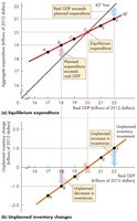
Actual vs. Planned Expenditure
Actual Expenditure: Always equals real GDP.
Planned Expenditure: May differ from actual expenditure due to unplanned inventory changes.
Equilibrium: Achieved when planned expenditure equals real GDP and inventories are stable.
Convergence to Equilibrium
If planned expenditure exceeds real GDP, inventories fall, prompting firms to increase production.
If real GDP exceeds planned expenditure, inventories rise, prompting firms to cut production.
The Multiplier Effect
Definition and Process
The multiplier measures how much equilibrium GDP changes in response to a change in autonomous expenditure. The effect is magnified because each round of spending induces further rounds of consumption.
Multiplier Formula: (in a simple closed economy)
Example: If , then .
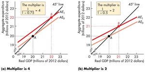
Key Insight: The higher the MPC, the larger the multiplier. Imports and taxes reduce the multiplier by causing some spending to leak out of the domestic economy.
Business Cycle Turning Points
Role of Autonomous Expenditure
Expansion: Triggered by an increase in autonomous expenditure, leading to unplanned inventory decreases and higher output.
Recession: Triggered by a decrease in autonomous expenditure, leading to unplanned inventory increases and lower output.
Aggregate Demand Curve and Price Level Changes
Deriving the Aggregate Demand Curve
Changes in the price level affect aggregate planned expenditure through wealth and substitution effects, shifting the aggregate expenditure curve and changing equilibrium GDP. A higher price level reduces equilibrium expenditure, moving the economy along the aggregate demand (AD) curve.
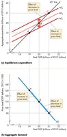
Shifts in AE and AD Curves
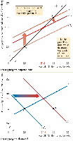
Increase in Investment: Shifts both AE and AD curves rightward by the change in investment times the multiplier.
Flat SRAS: If short-run supply is flat, the price level change is negligible.
Upward-Sloping SRAS: If SRAS slopes up, an increase in investment raises both output and the price level, but the multiplier is smaller than with fixed prices.
Summary Table: Key Marginal Propensities and Their Effects
Concept | Definition | Formula | Example Value |
|---|---|---|---|
Marginal Propensity to Consume (MPC) | Fraction of extra income spent on consumption | 0.75 | |
Marginal Propensity to Save (MPS) | Fraction of extra income saved | 0.25 | |
Multiplier | Change in equilibrium GDP per $1 change in autonomous expenditure | 4 (if MPC = 0.75) | |
Marginal Propensity to Import | Fraction of extra income spent on imports | n/a | 0.25 |
