IS-LM Model, Financial Crisis, and the Phillips Curve: Advanced Macroeconomics Study Notes

IS-LM Model

Introduction to the IS-LM Model

The IS-LM model is a foundational framework in macroeconomics that describes the joint equilibrium in the goods and money markets. It determines the equilibrium levels of national income (output, Y) and the interest rate (i) by considering the interactions between aggregate demand and monetary policy.

• Goods Market (IS Curve): Equilibrium where investment equals savings. Output is determined by aggregate expenditure, which depends on income and the interest rate.

• Money Market (LM Curve): Equilibrium where money demand equals money supply. The interest rate is determined by the central bank's policy and the demand for money, which is a function of income.

• Endogeneity: Investment is modeled as endogenous to both income and the interest rate: $I = I(Y, i)$.

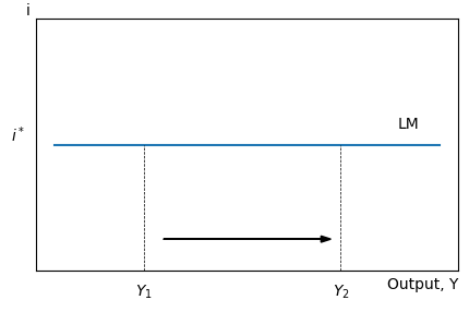
The LM Curve

The LM curve represents combinations of income and interest rates where the money market is in equilibrium. In modern central banking, the LM curve is often depicted as flat, reflecting the central bank's interest rate target.

• Flat LM Curve: The central bank adjusts the money supply to maintain its target interest rate ($i^*$), regardless of changes in income.

• Shifts in LM: Occur when the central bank changes its interest rate target (expansionary or contractionary monetary policy).

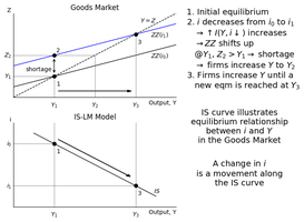
The IS Curve

The IS curve shows combinations of output and interest rates where the goods market is in equilibrium. It is downward sloping because lower interest rates stimulate investment and thus increase output.

• Endogenous Investment: $I = I(Y, i)$, so both higher income and lower interest rates increase investment.

• Shifts in IS: Occur due to changes in government spending (G), taxes (T), or autonomous consumption ($c_0$).

The Global Financial Crisis

Overview and Causes

The Global Financial Crisis (GFC) of 2007-2009 was a severe worldwide economic crisis. It was triggered by the collapse of the housing bubble in the United States, fueled by excessive credit, subprime lending, and financial innovations such as mortgage-backed securities (MBS).

• Housing Bubble: Rapid increase in home prices, followed by a sharp correction.

• Subprime Mortgages: High-risk loans to borrowers with low credit scores.

• Financial Innovations: Securitization (MBS, CDOs), credit default swaps (CDS), and structured investment vehicles (SIVs).

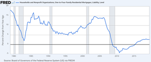
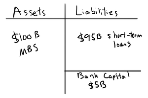
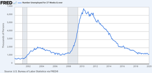
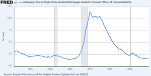
Mortgage Delinquency and Bank Balance Sheets

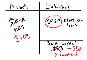
As home prices fell, mortgage delinquencies surged, especially among subprime borrowers. This led to a decline in the value of MBS and threatened the solvency of financial institutions.

• Delinquency Rate: The percentage of mortgages past due increased dramatically after the bubble burst.

• Balance Sheet Insolvency: When asset values fall below liabilities, banks become insolvent.

Policy Responses

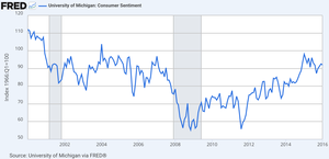
Governments and central banks responded with aggressive monetary and fiscal policies to stabilize the economy and restore confidence in the financial system.

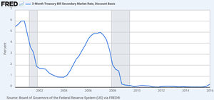
• Monetary Policy: Central banks lowered interest rates and engaged in quantitative easing.

• Fiscal Policy: Increased government spending and tax cuts.

• Other Measures: Asset purchases, bank bailouts, and guarantees.

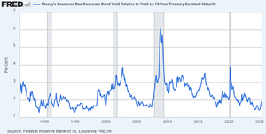
Risk Premiums and Financial Markets

During crises, risk and term premiums rise, increasing the cost of borrowing and shifting the IS curve leftward. Central banks can intervene to reduce these premiums by purchasing riskier assets.

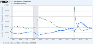
Labor Market and the Phillips Curve

Labor Market Equilibrium

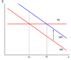
The labor market determines the natural rate of unemployment through the interaction of wage-setting and price-setting behavior. The equilibrium real wage is where the wage-setting (WS) and price-setting (PS) curves intersect.

• Wage Setting: $W = P^e F(u, z)$, where $W$ is the nominal wage, $P^e$ is expected price level, $u$ is unemployment rate, and $z$ captures other factors affecting bargaining power.

• Price Setting: $P = (1 + m)W$, where $m$ is the markup.

• Equilibrium Real Wage: $\frac{W}{P} = F(u, z) = \frac{1}{1 + m}$

Wage-Price Spiral

When actual prices exceed expected prices, workers demand higher wages, which firms pass on as higher prices, potentially leading to a wage-price spiral and persistent inflation.

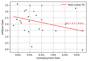
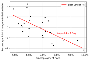
Phillips Curve: Theory and Evidence

The Phillips Curve describes the inverse relationship between inflation and unemployment. It is derived from the labor market model and can be expressed in both nonlinear and linearized forms.

• General Form: $\pi_t \approx \pi_t^e - \alpha u_t + m + z$

• Expectations: If expectations are anchored, the Phillips Curve predicts a negative correlation between inflation and unemployment. If expectations adapt to past inflation, the relationship is between changes in inflation and unemployment.

Empirical Evidence and Regression

The Phillips Curve is testable using regression analysis. The slope parameter $\alpha$ measures the sensitivity of inflation to unemployment, controlling for expected inflation and other factors.

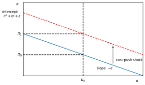
Medium-Run Equilibrium and Natural Rate of Unemployment

In the medium run, the natural rate of unemployment ($u_n$) is determined by structural factors and the markup. The Phillips Curve can be rewritten relative to equilibrium:

• Medium-Run Phillips Curve: $\pi_t - \pi^e = -\alpha (u_t - u_n)$

• If $u_t = u_n$, inflation is stable at the target. Deviations lead to rising or falling inflation.

Labor Market Data and the Phillips Curve

Empirical data show the relationship between wage growth, inflation, and unemployment over different periods. The Employment Cost Index (ECI) is a key measure of wage growth, and its relationship with unemployment is consistent with the Phillips Curve.

Summary Table: Key Equations and Relationships

Concept	Equation	Description
IS Curve	$Y = C(c_0, Y, T) + I(b_0, Y, i) + G$	Goods market equilibrium
LM Curve	$i = i^*$	Central bank interest rate target
Wage Setting	$W = P^e F(u, z)$	Nominal wage determination
Price Setting	$P = (1 + m)W$	Firm pricing with markup
Phillips Curve	$\pi_t \approx \pi_t^e - \alpha u_t + m + z$	Inflation-unemployment relationship
Medium-Run PC	$\pi_t - \pi^e = -\alpha (u_t - u_n)$	Deviation from natural rate

Additional info: These notes integrate theoretical models, empirical evidence, and policy responses, providing a comprehensive overview suitable for exam preparation in intermediate macroeconomics.