Macroeconomic Equilibrium, Gaps, and Fiscal Policy: Aggregate Demand and Supply Analysis

Aggregate Demand and Aggregate Supply Model

Overview of the AD-AS Model

The Aggregate Demand (AD) and Aggregate Supply (AS) model is a central framework in macroeconomics for analyzing fluctuations in output, employment, and the price level. It helps explain short-run and long-run economic changes, including business cycles, recessions, and expansions.

• Aggregate Demand (AD): Represents the total demand for goods and services in an economy at different price levels.

• Aggregate Supply (AS): Shows the total output firms are willing to produce at various price levels.

• Short-Run Aggregate Supply (SRAS): Reflects output when some prices or wages are sticky.

• Long-Run Aggregate Supply (LRAS): Indicates the economy's full potential output (Y*), where all resources are fully employed.

Key Variables: Real GDP, Price Level (CPI), Employment

Business Cycles and Economic Gaps

Full Potential and Output Gaps

Economic output fluctuates around its full potential (Y*) due to various shocks and policy interventions. Deviations from Y* are called output gaps:

• Recessionary Gap: Actual output (Y) is below potential output (Y*), indicating underutilized resources and higher unemployment.

• Inflationary Gap: Actual output (Y) exceeds potential output (Y*), leading to upward pressure on prices and lower unemployment.

Causes of Business Cycles

• Changes in aggregate demand (C, I, G, NX)

• Supply shocks (e.g., oil price increases, natural disasters)

• Expectations about future income and prices

Shifts and Movements in the AD and SRAS Curves

Shifts of the AD Curve

The AD curve shifts due to changes in its components:

• Consumption (C)

• Investment (I)

• Government Spending (G)

• Net Exports (NX)

For example, increased household expectations or improved business outlook can shift AD rightward, increasing output and price level.

Why is the AD Curve Downward Sloping?

• Wealth Effect: Higher price levels reduce real wealth, lowering consumption.

• Interest Rate Effect: Higher prices increase interest rates, reducing investment.

• International Trade Effect: Higher domestic prices reduce exports and increase imports.

Shifts of the SRAS Curve

The SRAS curve shifts due to changes in factor prices, productivity, and expectations:

• Increase in labor force (e.g., immigration)

• Improvements in education and productivity

• Changes in expected future prices

• Supply shocks (e.g., oil price spikes)

Why is the SRAS Curve Upward Sloping?

• Sticky wages and prices due to contracts

• Menu costs and slow adjustment by firms

• Difficulty predicting future prices

Macroeconomic Equilibrium and Adjustment

Short-Run and Long-Run Equilibrium

Equilibrium occurs where AD intersects SRAS (short run) and LRAS (long run). The economy adjusts to shocks over time as wages and prices respond.

Adjustment to Full Potential

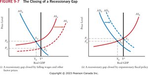
• In a recessionary gap, falling wages and prices shift SRAS right, restoring equilibrium at Y*.

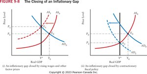
• In an inflationary gap, rising wages and prices shift SRAS left, bringing output back to Y*.

Fiscal Interventions

• Automatic Stabilizers: Progressive taxes and transfers that dampen fluctuations without new legislation.

• Discretionary Fiscal Policy: Deliberate changes in government spending or taxes to close output gaps.

Options for Closing a Recessionary Gap

There are two main approaches to closing a recessionary gap:

• Allow wages and factor prices to fall, shifting SRAS right.

• Use expansionary fiscal policy to shift AD right.

Options for Closing an Inflationary Gap

There are two main approaches to closing an inflationary gap:

• Allow wages and factor prices to rise, shifting SRAS left.

• Use contractionary fiscal policy to shift AD left.

Phillips Curve and Tradeoffs

Unemployment and Inflation

The Phillips Curve illustrates the short-run tradeoff between unemployment and inflation. Lower unemployment often comes with higher inflation, and vice versa.

Supply Side and Economic Growth

Factors Influencing Long-Run Growth

• Growth in the labor force

• Technological advancements

• Shifts in LRAS to the right indicate long-run economic growth

Static vs. Dynamic Models

Dynamic AD-AS Model

Dynamic models incorporate ongoing growth in real GDP, regular shifts in LRAS and AD, and changes in SRAS due to inflation expectations.

Saving Paradox

Short-Run vs. Long-Run Effects

• In the short run, increased saving reduces consumption and GDP.

• In the long run, higher saving boosts investment and potential GDP.

Key Equations

• Aggregate Demand: $AD = C + I + G + NX$

• Multiplier Effect: $\text{Multiplier} = \frac{1}{1 - MPC}$

• Output Gap: $\text{Output Gap} = Y - Y^*$

Example: If government increases spending (G), AD shifts right, potentially closing a recessionary gap and increasing real GDP and price level.

Additional info: Academic context and definitions have been expanded for clarity and completeness. Figures included are directly relevant to the explanation of closing recessionary and inflationary gaps using the AD-AS model.