Chapters 5-9 for final exam studying

Reconciling Macroeconomics and Microeconomics

Understanding the Scope of Economics

Macroeconomics and microeconomics are two branches of economics that analyze different levels of economic activity. While microeconomics focuses on the choices of individuals, households, businesses, and governments in specific markets, macroeconomics examines the performance of the entire economy, including national and global outcomes.

• Macroeconomics: Studies aggregate outcomes such as GDP, unemployment, and inflation, resulting from the sum of all microeconomic choices.

• Microeconomics: Analyzes individual decision-making and market interactions for goods, services, and resources.

• Fallacy of Composition: The error of assuming that what is true for an individual is true for the group; the whole can behave differently than the sum of its parts.

• Paradox of Thrift: If everyone tries to save more during a recession, aggregate demand falls, leading to lower total savings due to reduced income and employment.

The Circular Flow Model

The circular flow model simplifies the economy into three main players: households, businesses, and government. It illustrates how money, goods, services, and resources move through the economy.

• Input Markets: Where households provide resources (labour, capital, land) to businesses in exchange for income.

• Output Markets: Where businesses sell goods and services to households and government.

• Government: Collects taxes, provides public goods, and redistributes income.

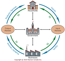
Microeconomics focuses on individual markets, while macroeconomics studies the connections between input and output markets, including the roles of money, banks, and expectations.

The Fundamental Macroeconomic Question

Debates in Macroeconomic Policy

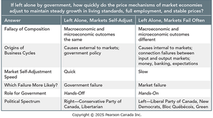
The central question in macroeconomics is: "If left alone by government, how quickly do market price mechanisms adjust to maintain steady growth, full employment, and stable prices?" There are two main schools of thought:

• Markets Self-Adjust (Hands-Off): Based on Say’s Law, which states that supply creates its own demand. Advocates minimal government intervention.

• Markets Fail Often (Hands-On): Based on Keynesian economics, which argues that markets can fail and require government intervention to stabilize the economy.

Economics and Politics

Political ideologies often align with these economic perspectives:

• Market Failure: Occurs when market outcomes are inefficient or inequitable.

• Government Failure: Occurs when government policies do not serve the public interest.

Comparing Hands-Off and Hands-On Approaches

Answer	Left Alone, Markets Self-Adjust	Left Alone, Markets Fail Often
Fallacy of Composition	Macroeconomic and microeconomic outcomes the same	Macroeconomic and microeconomic outcomes different
Origins of Business Cycles	External to markets; government policy	Connection failures between input/output markets, money, banking, expectations
Market Self-Adjustment Speed	Quick	Slow
Which Failure More Likely?	Government failure	Market failure
Role for Government	Hands-Off	Hands-On
Political Spectrum	Right—Conservative, Libertarian	Left—Liberal, NDP, Bloc, Green

Macroeconomic Outcomes and Players

Measuring Good Outcomes

Macroeconomic performance is evaluated by three main indicators:

• Higher GDP: Indicates steady growth in living standards.

• Lower Unemployment: Reflects full employment.

• Low and Predictable Inflation: Ensures stable prices.

Key Economic Players

• Consumers: Decide how much to spend or save, and whether to buy domestic or imported goods.

• Businesses: Make investment decisions, hire workers, and choose between domestic and imported inputs.

• Government: Purchases goods and services, sets fiscal policy (taxes and transfers).

• Banks and Bank of Canada: Influence the economy through loans and monetary policy (interest rates, money supply).

• Rest of World (R.O.W.): Engages in trade and investment with Canada.

Measuring GDP and Living Standards

Nominal vs. Real GDP

Gross Domestic Product (GDP) measures the value of all final goods and services produced within a country’s borders in a given year.

• Nominal GDP: Valued at current prices; changes can reflect price or quantity changes.

• Real GDP: Valued at constant prices; changes reflect only quantity changes.

• GDP per Person: Real GDP divided by population; best measure of material living standards.

• GDP is a flow: Measured per unit of time (e.g., per year).

• Stock: A fixed amount at a point in time (e.g., wealth).

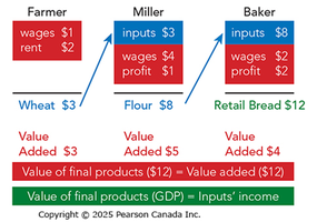
Value Added and the Circular Flow

Value added is the value of output minus the value of intermediate goods. It prevents double counting in GDP calculations.

• Value of Final Products and Services = Value Added

• GDP can be measured by total spending or total income: Aggregate spending (GDP) = Aggregate income (Y)

Components of the Enlarged Circular Flow

• C (Consumption): Spending by consumers

• I (Investment): Business spending on capital goods

• G (Government): Government spending on goods and services

• X (Exports): Foreign spending on Canadian goods/services

• IM (Imports): Canadian spending on foreign goods/services

Limitations of GDP as a Measure of Well-Being

• Excludes non-market production (e.g., household work)

• Misses underground economy (unreported or illegal activity)

• Ignores environmental sustainability

• Does not account for leisure or political freedoms

Potential GDP and Economic Growth

Potential GDP

Potential GDP is the maximum output an economy can produce when all resources are fully employed. It represents the short-run goal for economic performance and is the outcome if markets function perfectly.

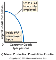
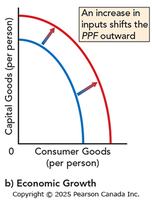
Economic Growth and the Production Possibilities Frontier (PPF)

Economic growth is the expansion of an economy’s capacity to produce goods and services, shown by an outward shift of the macro PPF.

• On the PPF: All inputs are fully employed (potential GDP).

• Inside the PPF: Some resources are unemployed (actual GDP below potential).

Growth is driven by increases in the quantity or quality of labour, capital, land/resources, and entrepreneurship, including technological change.

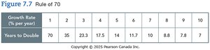
Rule of 70

The Rule of 70 estimates the number of years it takes for a variable to double, given a constant growth rate:

• Formula: $\text{Years to Double} = \frac{70}{\text{Annual Growth Rate (%)}}$

Growth Rate (% per year)	1	2	3	4	5	6	7	8	9	10
Years to Double	70	35	23.3	17.5	14	11.7	10	8.8	7.8	7

Productivity and Creative Destruction

• Productivity: Real GDP produced per hour of labour; higher productivity raises living standards.

• Creative Destruction: Innovation improves living standards but can eliminate outdated industries and jobs.

Business Cycles and Economic Shocks

Phases of the Business Cycle

• Expansion: Real GDP increases

• Peak: Highest point of expansion

• Contraction: Real GDP decreases

• Trough: Lowest point of contraction

• Recession: Two or more consecutive quarters of declining real GDP

Output Gap: Difference between real GDP and potential GDP

• Recessionary Gap: Real GDP below potential (negative gap)

• Inflationary Gap: Real GDP above potential (positive gap)

Economic Shocks

• External Shocks: Events outside the economy (e.g., natural disasters, wars, global price changes)

• Internal Shocks: Changes in expectations, financial disruptions, or market failures within the economy

• Shocks can be positive (expansionary) or negative (recessionary)

Unemployment: Measurement and Types

Calculating the Unemployment Rate

• Employed: Working for pay (full or part-time)

• Unemployed: Not working but actively seeking work

• Not in Labour Force: Not employed or seeking work (students, retirees)

• Labour Force: Employed + Unemployed

• Unemployment Rate: $\text{Unemployment Rate} = \frac{\text{Unemployed}}{\text{Labour Force}} \times 100$

• Labour Force Participation Rate: $\text{Labour Force Participation Rate} = \frac{\text{Labour Force}}{\text{Working-Age Population}} \times 100$

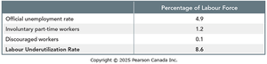
The official unemployment rate may understate true unemployment by excluding involuntary part-time and discouraged workers. The Labour Underutilization Rate includes these groups.

	Percentage of Labour Force
Official unemployment rate	4.9
Involuntary part-time workers	1.2
Discouraged workers	0.1
Labour Underutilization Rate	8.6

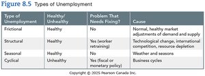
Types of Unemployment

Type	Healthy/Unhealthy	Problem That Needs Fixing?	Cause
Frictional	Healthy	No	Normal market turnover
Structural	Healthy	Yes (retraining)	Technological change, competition
Seasonal	Healthy	No	Weather, seasons
Cyclical	Unhealthy	Yes (policy)	Business cycles

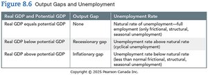
Output Gaps and Unemployment

Real GDP and Potential GDP	Output Gap	Unemployment Rate
Real GDP equals potential GDP	None	Natural rate (frictional, structural, seasonal only)
Real GDP below potential GDP	Recessionary gap	Above natural rate (cyclical unemployment)
Real GDP above potential GDP	Inflationary gap	Below natural rate

Inflation: Causes and Consequences

What Is Inflation?

• Inflation: Persistent rise in average prices, reducing the value of money.

• Consumer Price Index (CPI): Measures average prices of a fixed basket of goods and services (base year = 2002, CPI = 100).

• Inflation Rate: Annual percentage change in CPI.

• Core Inflation Rate: Excludes volatile items for a clearer trend.

Effects of Inflation

• Reduces purchasing power, especially for those with fixed incomes or savings.

• Creates uncertainty, discouraging investment.

• Bank of Canada targets 1–3% inflation for predictability.

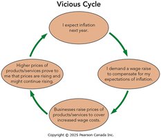
• Expectations of inflation can create a self-fulfilling cycle.

Disinflation and Deflation

• Disinflation: Slower rise in average prices (lower inflation rate).

• Deflation: Persistent fall in average prices (negative inflation rate); can lead to postponed spending and higher unemployment.

The Quantity Theory of Money

• Equation: $M \times V = P \times Q$

• M: Money supply

• V: Velocity of money

• P: Price level (CPI)

• Q: Real output (real GDP)

• "Printing money causes inflation" if output is at potential GDP and velocity is stable.

Unemployment and Inflation Trade-Offs

The Phillips Curve

• Shows inverse relationship between unemployment and inflation (short run).

• Demand-pull inflation: Caused by increased demand, leading to lower unemployment and higher prices.

• Cost-push inflation: Caused by supply shocks, leading to higher prices and higher unemployment (stagflation).

• Long-run Phillips Curve may flatten due to changing expectations and natural rate of unemployment.

Aggregate Supply and Aggregate Demand

Potential GDP and Long-Run Aggregate Supply (LAS)

• Potential GDP: Modeled as a point on the PPF and as a vertical LAS curve.

• LAS: Quantity of real GDP supplied when all inputs are fully employed; does not change with price level.

Short-Run Aggregate Supply (SAS)

• Shows planned supply of real GDP at different price levels, with some input prices fixed.

• As price level rises, quantity supplied increases (movement along SAS).

• Changes in input quantity/quality shift both LAS and SAS; changes in input prices shift only SAS.

Aggregate Demand (AD)

• Planned spending by all macroeconomic players at different price levels.

• As price level rises, aggregate quantity demanded decreases (movement along AD).

• Components: C (consumption), I (investment), G (government), X (exports), IM (imports).

• Demand shocks shift the AD curve (expectations, interest rates, government policy, foreign GDP, exchange rates).

Macroeconomic Equilibrium and Shocks

Short-Run and Long-Run Equilibrium

• Short-run equilibrium: Where SAS and AD intersect (with existing inputs).

• Long-run equilibrium: Where SAS, AD, and LAS all intersect (real GDP = potential GDP).

Economic Growth and Shifting Equilibrium

• Business investment increases inputs, shifting SAS and LAS rightward, raising potential GDP and living standards.

• Aggregate demand also shifts rightward as incomes rise.

Aggregate Demand and Supply Shocks

• Negative demand shock: Causes recessionary gap (lower prices, lower GDP, higher unemployment).

• Positive demand shock: Causes inflationary gap (higher prices, higher GDP, lower unemployment).

• Negative supply shock: Causes stagflation (higher prices, lower GDP, higher unemployment).

• Positive supply shock: Lowers prices, increases GDP, maintains full employment.

Using the AS/AD Model

To analyze economic events, start from long-run equilibrium and model shocks as shifts in AD or AS. Examine the effects on real GDP, unemployment, and inflation. Policy debates focus on how quickly the economy returns to equilibrium and the appropriate role for government intervention.