Macroeconomics and Microeconomics: Foundations, Models, and Key Outcomes

Reconciling Macroeconomics and Microeconomics

Definitions and Scope

Macroeconomics and microeconomics are two main branches of economics, each focusing on different levels of analysis:

• Macroeconomics analyzes the performance of the entire economy, including national and global outcomes, by aggregating the choices of all individuals, businesses, and governments.

• Microeconomics studies the choices made by individual households, businesses, and governments, and how these choices interact in specific markets.

• Fallacy of Composition: The error of assuming that what is true for one individual or part is true for the whole. For example, the Paradox of Thrift states that if everyone tries to save more, total savings may actually decrease due to reduced incomes and employment.

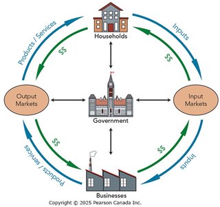
The Circular Flow Model

The circular flow model simplifies the economy into three main players: households, businesses, and governments. It illustrates how money, goods, services, and resources flow between these groups through input and output markets.

• Input markets determine incomes (e.g., wages, rent, profit).

• Output markets determine the value of all products and services sold.

• Microeconomics focuses on either input or output markets, while macroeconomics studies the connections between them, including the roles of money, banks, and expectations.

The Fundamental Macroeconomic Question

Market Adjustment and Policy Debates

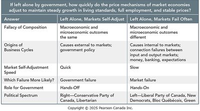
The central question in macroeconomics is: If left alone by government, how quickly do market price mechanisms adjust to maintain steady growth in living standards, full employment, and stable prices? There are two main schools of thought:

• Markets Self-Adjust (Hands-Off): Based on Say’s Law (supply creates its own demand), this view holds that markets adjust quickly and government intervention is usually unnecessary or harmful.

• Markets Fail Often (Hands-On): Following Keynesian economics, this view argues that markets can adjust slowly, business cycles are caused by failures in market connections, and government intervention is often needed to stabilize the economy.

Economics and Politics

• Market failure: When market outcomes are inefficient or inequitable.

• Government failure: When government policies fail to serve the public interest.

Comparing Hands-Off and Hands-On Approaches

Answer	Left Alone, Markets Self-Adjust	Left Alone, Markets Fail Often
Fallacy of Composition	Macro and micro outcomes the same	Macro and micro outcomes different
Origins of Business Cycles	External events or government policy	Connection failures, money, banking, expectations
Market Self-Adjustment Speed	Quick	Slow
Which Failure More Likely?	Government failure	Market failure
Role for Government	Hands-Off	Hands-On
Political Spectrum	Right—Conservative, Libertarian	Left—Liberal, Social Democrat

Macroeconomic Outcomes and Players

Measuring Good Outcomes

Macroeconomic performance is evaluated using three main indicators:

• Gross Domestic Product (GDP): Higher GDP per person indicates higher living standards.

• Unemployment: Lower unemployment is associated with full employment.

• Inflation: Low and predictable inflation is linked to stable prices.

Key Economic Players

• Consumers: Decide how much to spend or save, and whether to buy domestic or imported goods.

• Businesses: Make investment decisions, hire workers, and choose between domestic and imported inputs and outputs.

• Government: Purchases goods and services, sets fiscal policy (taxes, transfers, spending).

• Banks and Bank of Canada: Provide loans and conduct monetary policy (interest rates, money supply).

• Rest of World (R.O.W.): Engages in trade and investment with Canada.

GDP: Nominal, Real, and Value Added

Nominal vs. Real GDP

• Nominal GDP: The value of all final goods and services produced within a country in a year, measured at current prices.

• Real GDP: The value of all final goods and services produced, measured at constant prices (removing the effect of inflation).

• Real GDP per person: Real GDP divided by the population; best measure of material living standards.

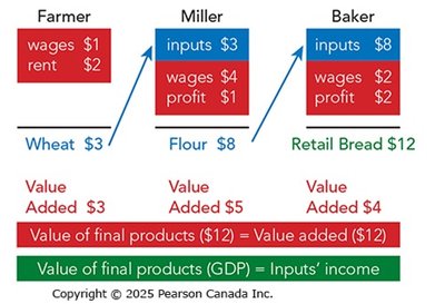
Value Added and the Circular Flow

• Value added: The value of output minus the value of intermediate goods and services purchased from other businesses. This avoids double counting in GDP calculation.

• GDP can be measured as either total spending on final goods and services or total income to input owners.

Enlarging the Circular Flow

Components of Spending

• C: Consumption spending by households

• I: Investment spending by businesses

• G: Government spending on goods and services

• X: Exports (spending by R.O.W. on Canadian goods/services)

• IM: Imports (Canadian spending on foreign goods/services)

Limitations of GDP as a Measure of Well-Being

• Excludes non-market production (e.g., household work)

• Misses underground economy (unreported or illegal activity)

• Does not account for environmental sustainability

• Ignores leisure and distribution of income, political freedoms, and social justice

Potential GDP and Economic Growth

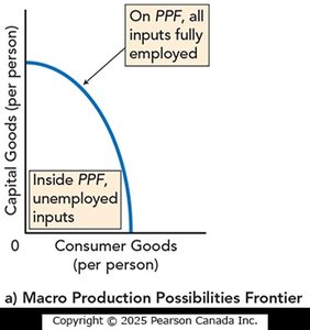
Potential GDP

• Potential GDP: The level of real GDP when all inputs (labour, capital, land, entrepreneurship) are fully employed.

• Represents the short-run maximum possible material living standards for an economy.

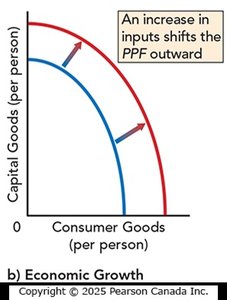
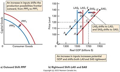
Economic Growth and the Production Possibilities Frontier (PPF)

• Economic growth: Expansion of the economy’s capacity to produce, shown as an outward shift of the macro PPF.

• Growth is driven by increases in the quantity or quality of inputs, including technological change.

Sources of Economic Growth

• Labour: Population growth, immigration, higher participation, and improved human capital (education, training).

• Capital: More factories/equipment and technological innovation.

• Land/Resources: Bringing new resources into use and improving their productivity.

• Entrepreneurship: Better management, organization, and innovation.

Measuring Economic Growth

• Economic growth rate: Annual percentage change in real GDP per person.

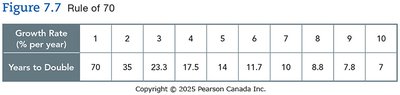
• Rule of 70: Years to double = 70 / (annual growth rate in percent).

Productivity and Creative Destruction

• Productivity: Real GDP produced per hour of labour; higher productivity raises living standards.

• Creative destruction: Innovation improves living standards but can eliminate less productive jobs and industries.

Business Cycles and Economic Shocks

Phases of the Business Cycle

• Expansion: Real GDP increases

• Peak: Highest point of expansion

• Contraction: Real GDP decreases

• Trough: Lowest point of contraction

• Recession: Two or more consecutive quarters of declining real GDP

Output Gaps

• Output gap: Real GDP minus potential GDP

• Recessionary gap: Real GDP below potential GDP (negative gap)

• Inflationary gap: Real GDP above potential GDP (positive gap)

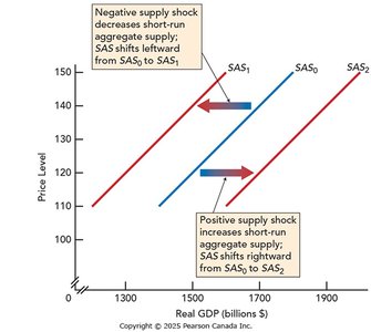
Economic Shocks

• External shocks: New technologies, resource discoveries, natural disasters, wars, policy changes

• Internal shocks: Changing expectations, financial market disruptions, failures in market connections

• Shocks can be positive (expansion) or negative (recession)

Unemployment: Measurement and Types

Measuring Unemployment

• Statistics Canada classifies the working-age population as employed, unemployed (actively seeking work), or not in the labour force.

• Labour Force = Employed + Unemployed

• Unemployment Rate = (Unemployed / Labour Force) × 100%

• Labour Force Participation Rate = (Labour Force / Working-Age Population) × 100%

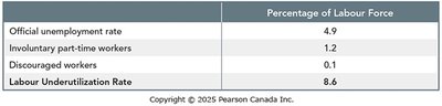
• Labour Underutilization Rate: Includes unemployed, involuntary part-time, and discouraged workers.

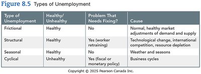
Types of Unemployment

Type	Healthy/Unhealthy	Needs Fixing?	Cause
Frictional	Healthy	No	Normal job search and turnover
Structural	Healthy	Yes (retraining)	Technological change, competition
Seasonal	Healthy	No	Weather, seasons
Cyclical	Unhealthy	Yes (policy)	Business cycles

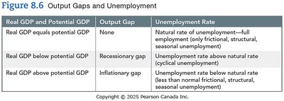
Output Gaps and Unemployment

Real GDP and Potential GDP	Output Gap	Unemployment Rate
Real GDP equals potential GDP	None	Natural rate (frictional, structural, seasonal)
Real GDP below potential GDP	Recessionary gap	Above natural rate (cyclical unemployment)
Real GDP above potential GDP	Inflationary gap	Below natural rate

Inflation: Causes and Consequences

Definition and Measurement

• Inflation: Persistent rise in average prices and fall in the value of money.

• Consumer Price Index (CPI): Measures average prices of a fixed basket of goods and services; base year CPI = 100.

• Inflation Rate: Annual percentage change in CPI.

• Core Inflation Rate: Excludes volatile categories for a clearer trend.

Effects of Inflation

• Reduces purchasing power, especially for those with fixed incomes or savings.

• Creates uncertainty, discouraging investment.

• Bank of Canada targets 1–3% inflation for predictability.

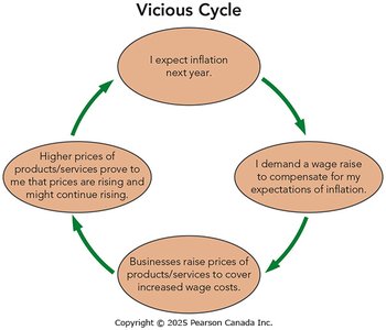
• Expectations of inflation can create a self-fulfilling cycle.

Disinflation and Deflation

• Disinflation: Decrease in the inflation rate (prices rise more slowly).

• Deflation: Persistent fall in average prices (negative inflation rate); can cause economic contraction and higher unemployment.

The Quantity Theory of Money

• Equation: $M \times V = P \times Q$ Where:

  • M = Money supply

  • V = Velocity of money

  • P = Price level (CPI)

  • Q = Real output

• If V and Q are constant, increases in M cause proportional increases in P (inflation).

Unemployment and Inflation Trade-Offs

The Phillips Curve

• Shows an inverse relationship between unemployment and inflation (short run).

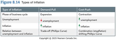
• Demand-pull inflation: Caused by increased demand; leads to lower unemployment and higher inflation.

• Cost-push inflation: Caused by decreased supply (e.g., supply shocks); leads to higher unemployment and higher inflation (stagflation).

Type of Inflation	Demand-Pull	Cost-Push
Phase of Business Cycle	Expansion	Contraction
Unemployment	Decreases	Increases
Inflation	Increases	Increases
Relation	Trade-off (Phillips Curve)	Stagflation (shifting Phillips Curve)

Aggregate Supply and Aggregate Demand

Potential GDP and Long-Run Aggregate Supply (LAS)

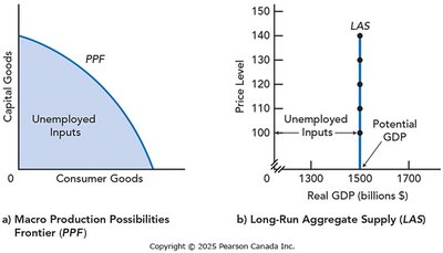
• Potential GDP: Modeled as points on the PPF and the vertical LAS curve.

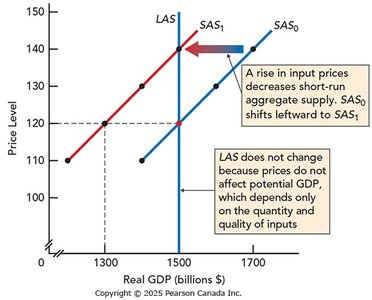
• LAS is vertical at potential GDP; does not change with price level.

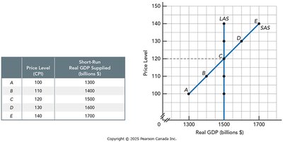
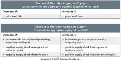
Short-Run Aggregate Supply (SAS)

• SAS shows the quantity of real GDP supplied at different price levels, with some input prices fixed.

• As price level rises, aggregate quantity supplied increases (movement along SAS).

• Changes in input quantity/quality shift both LAS and SAS; changes in input prices shift only SAS.

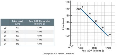
Aggregate Demand (AD)

• AD shows the quantity of real GDP demanded at different price levels by all macroeconomic players.

• As price level rises, aggregate quantity demanded decreases (movement along AD).

• AD is composed of C, I, G, and (X – IM).

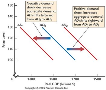
Demand Shocks

• Factors other than price (expectations, interest rates, government policy, foreign GDP, exchange rates) can shift the AD curve.

• Negative demand shocks shift AD left; positive shocks shift AD right.

Macroeconomic Equilibrium

Short-Run and Long-Run Equilibrium

• Short-run equilibrium: Intersection of SAS and AD.

• Long-run equilibrium: Intersection of SAS, AD, and LAS; real GDP equals potential GDP.

• Economic growth shifts LAS, SAS, and AD rightward, raising living standards with stable prices.