Macroeconomics Study Guide: Unemployment, Inflation, Economic Growth, and the AS-AD Model

Unemployment and Inflation

The Labor Market and Unemployment

The labor market is a central focus in macroeconomics, as it determines employment, unemployment, and related indicators. Unemployment results in lost incomes and production, and can pause human capital accumulation. Some unemployment is inevitable, even in full-employment economies, due to labor market turnover and creative destruction.

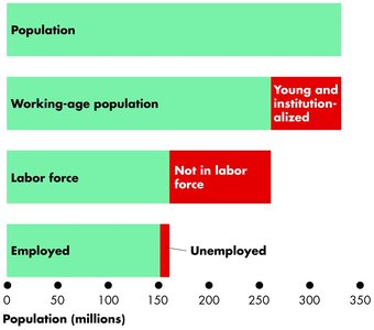
• Working-age population: People aged 16 and older, not in institutions.

• Labor force: Sum of employed and unemployed workers.

• Unemployed: Includes those actively seeking work, waiting to be recalled, or waiting to start a new job.

Labor Market Indicators

• Unemployment rate: $\text{Unemployment Rate} = \frac{\text{Unemployed Workers}}{\text{Labor Force}}$

• Labor force participation rate: $\text{Labor Force Participation Rate} = \frac{\text{Labor Force}}{\text{Working-age Population}}$

• Employment/population ratio: Measures employed as a fraction of working-age population.

Types of Unemployment

• Frictional unemployment: Arises from normal labor market turnover; healthy for a growing economy.

• Structural unemployment: Caused by changes in technology or competition; lasts longer and increases the natural rate of unemployment.

• Cyclical unemployment: Occurs during recessions when GDP is below potential; can be negative in overheated economies.

Inflation and Deflation

Inflation is the rise in prices, acting as a regressive tax and disrupting credit markets. Hyperinflation can devastate economies. Deflation, or falling prices, is also problematic, leading to delayed purchases and economic contraction.

Measuring Inflation: The Consumer Price Index (CPI)

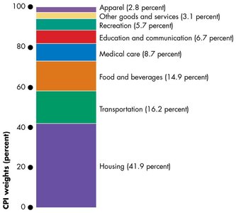
The CPI measures the average price level of a fixed basket of goods and services. It is set to 100 for the base period (1982-1984). The CPI basket is based on consumer expenditure surveys.

Calculating the CPI

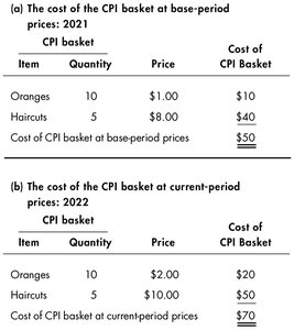
• Hold quantities constant, compare costs at different prices.

• $\text{CPI} = \frac{\text{Cost of CPI basket in current year}}{\text{Cost of CPI basket in base year}} \times 100$

• Example: If the basket cost $50 in 2021 and $70 in 2022, CPI = 140.

CPI Biases

• Overstates inflation by keeping the basket fixed and not adjusting for quality or new goods.

• Government transfers indexed to CPI may rise faster than needed.

Nominal and Real Interest Rates

• Nominal interest rate: Price of money now vs. future.

• Real interest rate: Price of goods/services now vs. future.

• $\text{Real Interest Rate} = \text{Nominal Interest Rate} - \text{Rate of Inflation}$

The Phillips Curve

The Phillips curve posits an inverse relationship between unemployment and inflation, though this relationship has become less clear in recent decades.

Economic Growth

Growth vs. Business Cycles

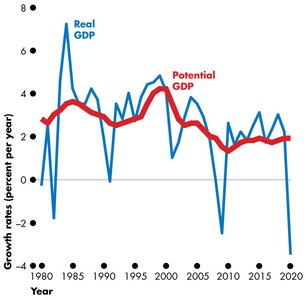
Economic growth studies the long-run evolution of potential GDP, while business cycles are short-run fluctuations around potential GDP. The growth rate of real GDP is:

• $\text{Growth Rate of } Y_{t+1} = \frac{Y_{t+1} - Y_t}{Y_t}$

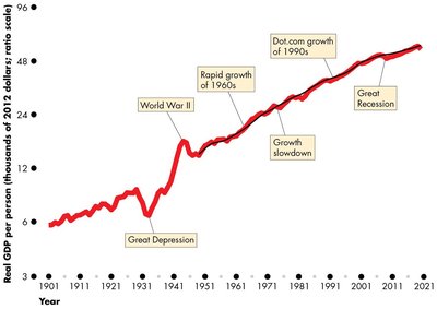
Long-Term US Economic Growth

• Average per capita growth of 2% over 1901-2021.

• Rule of 70: Years to double ≈ 70 / growth rate.

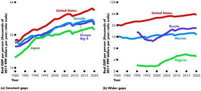
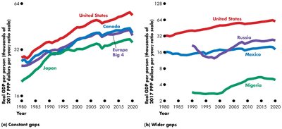
International Growth Comparisons

• Growth rates and income gaps vary across countries.

The Aggregate Production Function: Cobb-Douglas

The Cobb-Douglas production function describes how output (GDP) is produced with capital and labor:

• $Y = A K^{\alpha} N^{1-\alpha}$, where $A$ is total factor productivity (TFP), $\alpha$ is capital share.

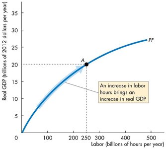
• Exhibits constant returns to scale and diminishing marginal returns.

Diminishing Marginal Returns

Increasing one input while holding the other constant yields smaller and smaller output gains.

The Labor Market and Equilibrium

• Labor demand is downward sloping due to diminishing returns.

• Labor supply is upward sloping; higher real wages attract more labor.

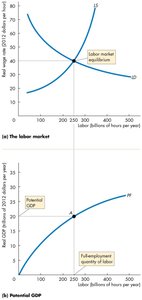
Sources of GDP Growth

• Growth in labor supply: More hours, higher employment/population ratio, population growth.

• Growth in labor productivity: Investment in physical and human capital, technological innovation.

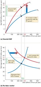
Investment and Productivity

• Physical capital: Increases productivity, but with diminishing returns.

• Human capital: Education, training, and experience raise productivity.

• Technological change: Drives long-run growth in GDP per capita.

Theories of Growth

• Malthusian theory: Pre-industrial economies were stuck in a poverty trap; population growth offset gains in living standards.

• Neoclassical growth: Sustained per capita growth is possible when population growth is moderate and TFP drives growth.

Capital, Convergence, and TFP

• Poor countries should grow faster due to higher returns on capital, but TFP is the key determinant of long-run growth.

• TFP depends on institutions, competition, public goods, and other factors.

The AS-AD Model

Aggregate Supply: Long Run and Short Run

• Long-run aggregate supply (LAS): Vertical; real GDP equals potential GDP.

• Short-run aggregate supply (SAS): Upward sloping; nominal wages are fixed, so higher prices increase supply.

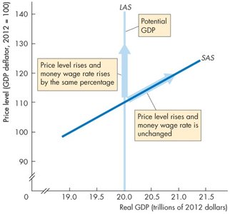
Price Adjustments and Equilibrium

• SAS and LAS curves intersect at potential GDP.

• As price level falls below equilibrium, real GDP supplied decreases.

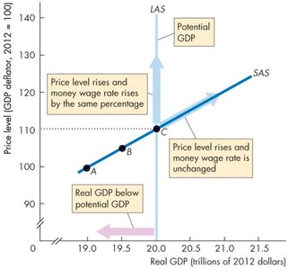
Changes in Aggregate Supply

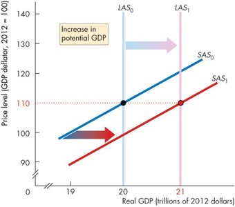
• Aggregate supply shifts due to changes in money wage rate, potential GDP, labor, capital, or technology.

Changes in Money Wage Rate

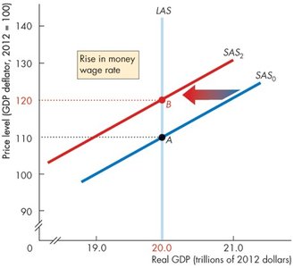
• Rise in money wage rate shifts SAS leftward; LAS does not change.

Aggregate Demand (AD)

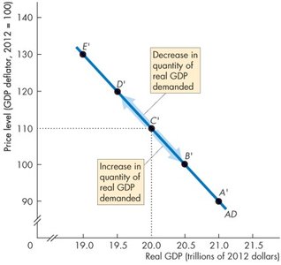
• AD is the relationship between real GDP demanded and the price level.

• AD curve slopes downward due to wealth and substitution effects.

Factors Shifting the AD Curve

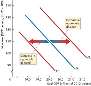
• Expectations, fiscal and monetary policy, and the world economy can shift AD.

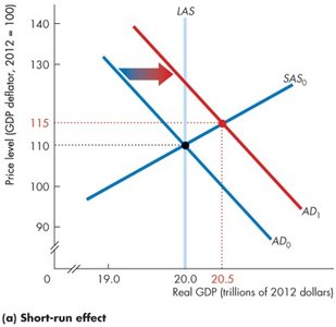
• Increase in AD shifts the curve rightward; decrease shifts it leftward.

Short-Run Macroeconomic Equilibrium

• Occurs where AD and SAS intersect; real GDP can be above or below potential GDP.

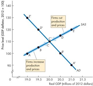
Long-Run Equilibrium

• Occurs when real GDP equals potential GDP at the intersection of AD and LAS.

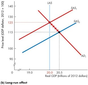
• Money wage adjusts over time to restore full employment.

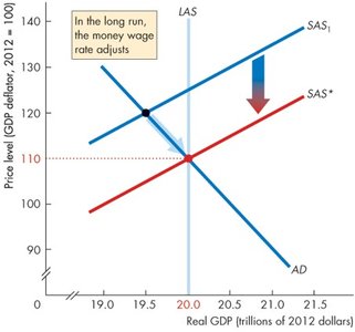
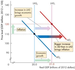
Growth and Inflation in the AS-AD Model

• LAS shifts right as potential GDP increases.

• If money supply grows faster than potential GDP, AD shifts right faster, causing inflation.

Business Cycles in the AS-AD Model

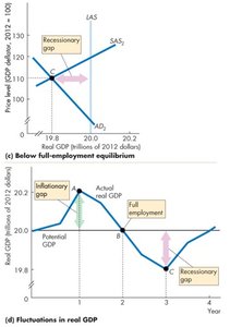
• Business cycles occur due to fluctuations in AD and SAS, with sticky wages preventing rapid adjustment.

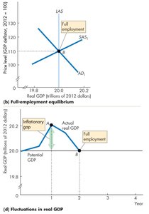
• Equilibrium can be above, at, or below full employment.

Return to Full Employment

• Inflationary gap: GDP above potential, unemployment below natural rate; wages rise, SAS shifts left.

• Recessionary gap: GDP below potential, unemployment above natural rate; wages fall, SAS shifts right.

Negative Supply Shock

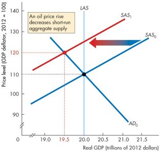
• SAS shifts leftward, real GDP decreases, price level rises; economy experiences stagflation.

Macroeconomic Schools of Thought

• Classical/Monetarist: Believe in self-correcting economy; minimal policy intervention.

• Keynesian/New-Keynesian: Advocate fiscal and monetary policy to manage business cycles.

Expenditure Multipliers

The Keynesian Model

• Prices are fixed; short-run aggregate supply is flat.

• Aggregate expenditure determines real GDP.

Autonomous and Induced Expenditure

• Autonomous: Investment (I), Government (G), Exports (X).

• Induced: Consumption (C), Imports (M), depend on income (Y).

Marginal Propensities

• MPC: Fraction of extra income spent on consumption.

• MPS: Fraction of extra income saved.

• MPC + MPS = 1

The Multiplier

• Change in equilibrium expenditure is larger than change in autonomous expenditure.

• $\text{Multiplier} = \frac{1}{1 - b}$, where $b$ is the slope of the aggregate expenditure curve.

• Imports and income taxes reduce the multiplier.

Business Cycle Turning Points

• Peaks and troughs occur when autonomous expenditure changes.

Aggregate Demand Curve Derivation

• Price level changes cause wealth and substitution effects, shifting aggregate planned expenditure and real GDP demanded.

Quantity and Price Effects

• Increase in investment shifts AE and AD curves rightward; price level rises, real GDP increases along SAS curve.

Additional info: All equations are provided in LaTeX format as required. Images included are directly relevant to the adjacent paragraphs and reinforce key concepts.