Phillips Curve and IS-LM-PC Model: Inflation, Unemployment, and Macroeconomic Shocks

Phillips Curve: Inflation and Unemployment

Basic Relationship and Graphical Derivation

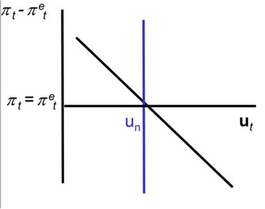
The Phillips Curve describes the relationship between the rate of inflation (πt) and the unemployment rate (ut). It shows that, for a given expected inflation (πet), an increase in unemployment leads to a decrease in inflation. When unemployment equals the natural rate (un), actual inflation matches expected inflation.

• Key Point: Higher unemployment reduces nominal wages, leading to lower price levels and inflation.

• Key Point: The Phillips Curve is not static; it shifts with changes in expectations and structural variables.

• Example: If wage setters expect higher prices, they demand higher nominal wages, causing firms to raise prices and inflation.

Versions of the Phillips Curve

There are several versions of the Phillips Curve, depending on how inflation expectations are formed:

• Original Phillips Curve: Assumes fixed inflation expectations.

• Accelerating Phillips Curve: Incorporates past inflation rates into expectations (parameter θ).

• Modern Phillips Curve: High current inflation increases the likelihood of high future inflation, leading to second-round effects.

Key Equations:

• $\pi_t = \pi^e_t - \alpha (u_t - u_n)$

• $\pi^e_t = \theta \pi_{t-1} + (1-\theta)\pi^*$

Additional info: θ measures the weight of past inflation in forming expectations; it increased during the 1970s, reflecting loss of central bank credibility.

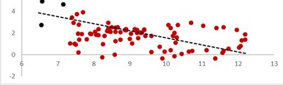
Empirical Evidence and Deviations

Empirical data sometimes show deviations from the Phillips Curve, especially during periods of supply shocks or when inflation expectations are not anchored.

• Example: In 2022-2023, inflation in the Eurozone was much higher than predicted by the traditional Phillips Curve.

Supply Shocks and Inflation

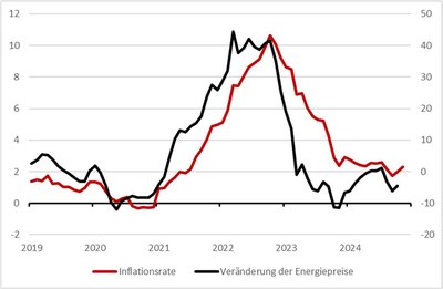
Covid-Inflation and Energy Price Shocks

Supply shocks, such as sudden increases in energy prices, can cause inflation independently of unemployment. These shocks raise input costs, prompting firms to increase prices.

• Key Point: The 1970s oil crises and recent post-Covid energy price surges are examples of supply shocks.

• Key Point: Such shocks can temporarily increase inflation, but their long-term effect depends on wage responses and inflation expectations.

• Example: The post-pandemic inflation was largely driven by energy and food price increases, not by wage-price spirals.

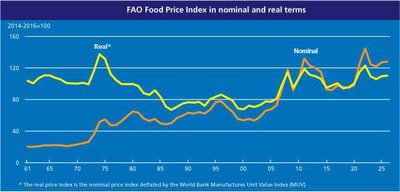
Food Price Index and Global Supply Chains

Global disruptions, such as wars or supply chain interruptions, can affect food prices and contribute to inflation. The FAO Food Price Index tracks these changes in both nominal and real terms.

• Key Point: Food price spikes can result from input cost increases, climate effects, and supply chain disruptions.

• Example: The Iran war scenario led to higher logistics and food prices, impacting inflation globally.

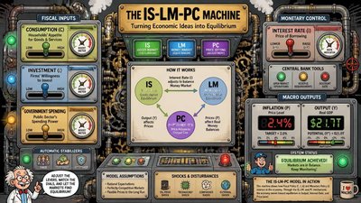
IS-LM-PC Model: Integrating Goods, Financial, and Labor Markets

Model Structure and Dynamics

The IS-LM-PC Model combines the goods market (IS), financial market (LM), and labor market (PC) to analyze macroeconomic equilibrium. It explains how output, unemployment, and inflation interact in the short and medium term.

• IS Curve: Output is determined by aggregate demand in the short run.

• LM Curve: Money market equilibrium determines the real interest rate.

• PC Curve: Inflation dynamics depend on the output gap and expectations.

• Key Point: In the short run, output can deviate from potential, causing inflation to rise or fall. In the medium run, output returns to potential, and inflation stabilizes.

Key Equations:

• $Y - Y_n = -L(u - u_n)$

• If $Y > Y_n$, inflation rises above expectations; if $Y < Y_n$, inflation falls below expectations.

Policy Implications and Adjustment Process

Central banks play a crucial role in stabilizing inflation and output. The adjustment to medium-term equilibrium depends on the accuracy of expectations and the speed of policy responses.

• Key Point: If inflation expectations are not anchored, persistent inflation can occur, requiring restrictive monetary policy.

• Key Point: Supply shocks (e.g., oil price increases) can cause stagflation—rising inflation and falling output.

• Example: The Iran war scenario illustrates how energy and food price shocks affect inflation, interest rates, and GDP.

Summary and Key Takeaways

• Phillips Curve: Shows the relationship between inflation, expected inflation, and unemployment. Its stability depends on how expectations are formed.

• Supply Shocks: Directly impact inflation, especially when expectations are not anchored.

• IS-LM-PC Model: Integrates goods, financial, and labor markets to explain macroeconomic dynamics and policy responses.

• Policy: Central bank credibility and anchored expectations are crucial for preventing inflation spirals and managing supply shocks.