Static One-Period Macroeconomic Model with Government: Equilibrium, Efficiency, and Policy Effects

Static One-Period Macroeconomic Model

Introduction to the Model

This chapter introduces a closed-economy, one-period macroeconomic model that incorporates a representative consumer, a representative firm, and the government. The model is used to analyze equilibrium, economic efficiency, and the effects of fiscal policy and productivity changes.

• Closed Economy: No trade with the outside world; exports (X), imports (M), and net exports (NX) are zero.

• Static Economy: Only one period; no saving, borrowing, or investment.

• Market Clearing: All goods produced must be consumed, and all labor supplied must be employed.

Model Structure: Exogenous and Endogenous Variables

The model distinguishes between exogenous variables (determined outside the model) and endogenous variables (determined within the model).

• Exogenous Variables: Government spending (G), total factor productivity (z), maximum hours (h), capital (K).

• Endogenous Variables: Consumption (C), labor supply (Ns), labor demand (Nd), taxes (T), profits (π), output (Y), real wage (w).

Market Clearing Conditions

Equilibrium requires that all markets clear:

• Goods Market: All goods produced (Y) are consumed by households (C) and government (G): $C + G = Y$

• Labor Market: Labor supply equals labor demand: $N_s = N_d$

• Price Mechanism: The real wage (w) is the only price in the model.

Government Budget Constraint

The government spends G and finances it through taxes T. In equilibrium:

• $G = T$

• Fiscal Policy: The government’s choice of G and T.

Competitive Equilibrium

A competitive equilibrium is an allocation and set of prices where all agents optimize and all markets clear. The equilibrium conditions are:

• Consumer utility maximization given w, T, h, π

• Firm profit maximization given w, z, K

• Government budget constraint: $G = T$

• Goods market: $C + G = Y$

• Labor market: $N_s = N_d$

Walras’ Law

If all but one market clears, the last market must also clear. In this model, labor market clearing implies goods market clearing.

• Consumer’s Budget Constraint: $C = wN_s + \pi - T$

• Firm Profits: $\pi = Y - wN_d$

• Substituting and using $N_s = N_d = N$ and $T = G$ yields $C + G = Y$

Production Possibilities Frontier (PPF)

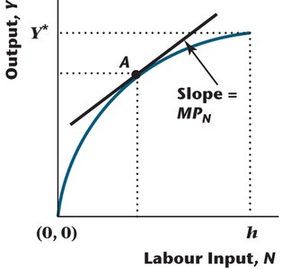
Production Function

The production function describes the relationship between labor input and output:

• $Y^* = zF(K, h)$: Maximum output when all available labor (h) is used.

• Marginal Product of Labor (MPN): The slope of the production function.

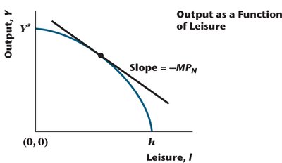
PPF as a Function of Leisure

By changing the horizontal axis to leisure ($l = h - N$), the production function becomes $zF(K, h - l)$.

• When $l = 0$, $N = h$, maximum output is produced.

• When $l = h$, $N = 0$, output is zero.

• The slope is $-MPN$.

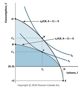
PPF with Consumption and Leisure

Changing the vertical axis to consumption ($C = Y - G$) shifts the production function downward. The PPF shows the trade-off between consumption and leisure.

• Maximum consumption is $Y^* - G$.

• The shaded area is the production possibilities set; the arc DA is the PPF.

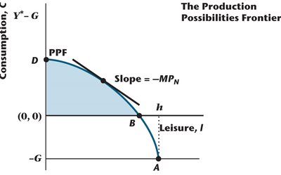
Marginal Rate of Transformation (MRT)

The negative slope of the PPF is the marginal rate of transformation (MRT), which equals the marginal product of labor (MPN):

• $MRT_{l,C} = MPN = -\text{slope of the PPF}$

• Describes the rate at which leisure can be converted into consumption goods.

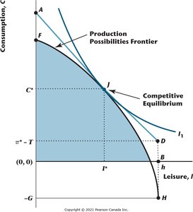
Equilibrium Analysis

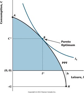
Graphical Analysis of Equilibrium

Equilibrium occurs where the consumer’s budget line is tangent to the PPF and the indifference curve:

• Firm optimization: $w = MPN = MRT_{l,C}$

• Consumer optimization: $MRS_{l,C} = w$

• In equilibrium: $MRT_{l,C} = MRS_{l,C}$

Pareto Optimality and Welfare Theorems

Pareto Optimality

An allocation is Pareto optimal if no one can be made better off without making someone else worse off. It is a criterion of economic efficiency.

• Social planner maximizes utility by choosing hours worked (N), allocating G to government, and $Y - G$ to consumer.

• No markets; centrally planned economy.

Finding the Pareto Optimal Allocation

The Pareto optimal allocation occurs where $MRS_{l,C} = MRT_{l,C} = MPN$.

• To the left of the optimal point: $MRT_{l,C} < MRS_{l,C}$ (can increase leisure).

• To the right: $MRT_{l,C} > MRS_{l,C}$ (can increase consumption).

First and Second Welfare Theorems

• First Welfare Theorem: Under certain conditions, a competitive equilibrium is Pareto optimal.

• Second Welfare Theorem: Under certain conditions, a Pareto optimum is a competitive equilibrium.

• Both theorems hold in this basic model.

Economic Inefficiencies

Factors that cause the welfare theorems to fail include:

• Externalities (pollution, education, public goods)

• Distortionary taxes (e.g., labor income tax)

• Monopoly power

• Information asymmetries (moral hazard, adverse selection)

• Government intervention may improve welfare in these cases.

Policy Experiments and Business Cycle Analysis

Experiment 1: Increase in Government Spending (G)

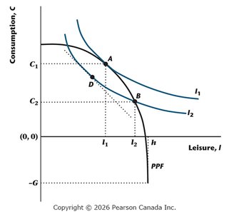
An increase in G shifts the PPF downward, increases taxes, and reduces both consumption and leisure (pure income effect).

• $C_2 < C_1$, $l_2 < l_1$

Crowding Out Effect

As leisure falls, labor supplied increases, raising output. Consumption is crowded out but not completely.

• $N_2 > N_1$, $Y_2 > Y_1$

• $\Delta C = \Delta Y - \Delta G$

Equilibrium Effects of Increased G

Firms demand more labor as the real wage falls. The income effect dominates, so consumers supply more labor.

• $w_2 < w_1$

Model Predictions: Government Spending

• Output (Y) and employment (N) increase (pro-cyclical).

• Consumption (C) and real wage (w) decrease (counter-cyclical).

• Business cycles are not likely driven by fluctuations in government spending.

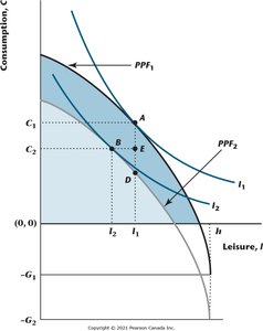
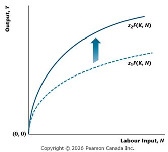
Experiment 2: Increase in Total Factor Productivity (z)

An increase in z shifts the production function up, increasing the marginal product of labor for each labor input.

• $Y = zF(K, N)$

Equilibrium Effects of Increased z

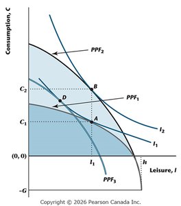
The PPF shifts outward, and the competitive equilibrium changes. Output, consumption, and real wage increase; leisure and employment may rise or fall.

• Income and substitution effects are involved.

Income and Substitution Effects

The effects of increased productivity are separated into substitution and income effects. The substitution effect is the movement along the PPF, while the income effect is the shift to a higher indifference curve.

• PPF1: Initial PPF

• PPF2: New PPF after productivity increase

• PPF3: Artificial PPF with income effect removed

Model Predictions: Productivity

• Output (Y), employment (N), consumption (C), and real wage (w) all increase (pro-cyclical).

• Business cycles are likely driven by fluctuations in total factor productivity.

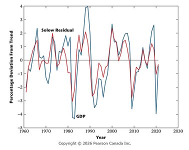
Empirical Evidence: Solow Residual and GDP

Percentage deviations from trend in the Solow residual (total factor productivity) and real GDP track each other closely, supporting the view that productivity fluctuations drive business cycles.

Distorting Taxes and Government Policy

Distorting Tax on Wage Income

A proportional tax on wage income causes the competitive equilibrium to be inefficient (not Pareto optimal). Labor supply and output are lower than at the Pareto optimum.

• Government budget constraint: $G = tw(h - l)$

• Consumer budget constraint: $C = w(1 - t)(h - l) + \pi$

• In equilibrium: $w(1 - t) = MRS_{l,c} < w = MPN = MRT_{l,c}$

Competitive Equilibrium with Distorting Tax

The PPF is unchanged, but the competitive equilibrium is at a point where the marginal rate of substitution is less than the marginal rate of transformation.

Examples: Lump-Sum vs. Proportional Taxes

Solving the consumer’s problem for utility $u(c, \ell) = \log(c) + A\ell$:

• Lump-Sum Tax: $c = w(h - \ell) + \pi - T$

• Proportional Tax: $c = (1 - \tau)w(h - \ell) + \pi$

First-order conditions yield:

• Lump-sum: $c_{LST} = w/A$, $\ell_{LST} = h - 1/A + (\pi - T)/w$

• Proportional: $c_{PIT} = (1 - \tau)w/A$, $\ell_{PIT} = h - 1/A + \pi/[(1 - \tau)w]$

• Consumption is lower under a proportional labor income tax than under a lump-sum tax: $c_{PIT} < c_{LST}$

Summary Table: Effects of Government Policy and Productivity

Policy/Change	Output (Y)	Employment (N)	Consumption (C)	Real Wage (w)
Increase in G	↑	↑	↓	↓
Increase in z	↑	↑/↓	↑	↑
Distorting Tax	↓	↓	↓	↓

Additional info: The above table summarizes the main effects of government spending, productivity, and distortionary taxes on macroeconomic variables in the static one-period model.