The Aggregate Demand and Aggregate Supply (AD/AS) Model: Structure, Shifts, and Macroeconomic Equilibrium

The AD/AS Model

Introduction to the AD/AS Model

The Aggregate Demand/Aggregate Supply (AD/AS) model is a fundamental framework in macroeconomics used to analyze the relationship between total spending (demand) and total production (supply) in an economy. It helps explain fluctuations in output, employment, and the price level, and is central to understanding business cycles and policy impacts.

Aggregate Demand (AD)

Definition and Components

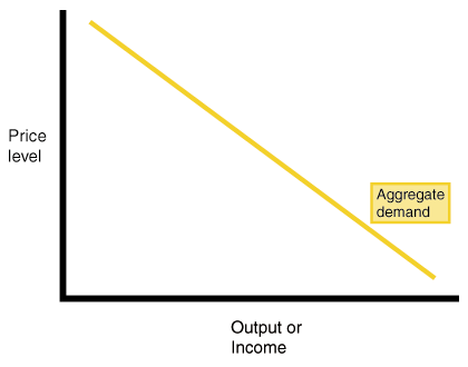
Aggregate demand (AD) is the total quantity of final goods and services demanded across all sectors of an economy at various price levels, during a given period. The main components of AD are:

• Consumption (C): Household spending on goods and services

• Investment (I): Business spending on capital goods

• Government Spending (G): Public sector expenditures

• Net Exports (NX): Exports minus imports

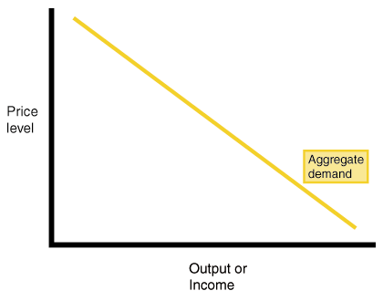
The AD curve shows a negative (downward) relationship between the price level and the quantity of output demanded.

Reasons for the Negative Slope of the AD Curve

• Wealth Effect: As the price level falls, the real value of money increases, encouraging more consumption.

• Interest Rate Effect: Lower price levels reduce interest rates, stimulating investment and consumption.

• Net Export Effect: A lower domestic price level makes exports more competitive, increasing net exports.

Shifts in the AD Curve

The AD curve shifts when factors other than the price level change, such as changes in consumption, investment, government spending, or net exports. For example, a tax cut increases disposable income, boosting consumption and shifting AD to the right.

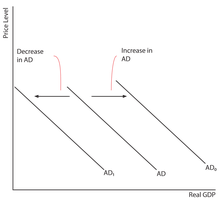
Other factors that can shift AD include changes in consumer confidence, interest rates, household wealth, and global economic conditions.

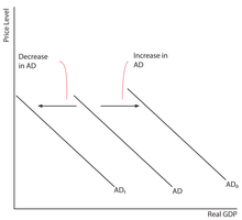
AD Curve During a Recession

During a recession, aggregate demand decreases, causing the AD curve to shift to the left. This results in lower real GDP and higher unemployment.

Aggregate Supply (AS)

Short-Run and Long-Run Aggregate Supply

There are two aggregate supply curves:

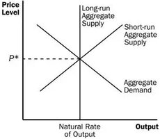
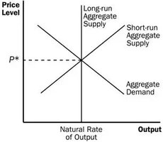
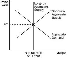
• Short-Run Aggregate Supply (SRAS): Positively sloped; shows the relationship between the price level and output supplied in the short run.

• Long-Run Aggregate Supply (LRAS): Vertical; represents the economy's maximum sustainable output (potential GDP) when all resources are fully employed.

Why SRAS is Upward Sloping

As output increases, firms require more resources, pushing up costs (especially wages). Higher costs lead to higher prices, resulting in the upward slope of the SRAS curve.

Shifts in the SRAS Curve

SRAS shifts due to changes in input prices (e.g., oil, wages), supply shocks (e.g., natural disasters), and changes in the availability of resources. A negative supply shock (e.g., a pandemic) shifts SRAS left, reducing output and increasing prices.

Shifts in the LRAS Curve

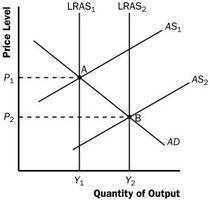
The LRAS curve shifts with changes in the economy's productive capacity, such as population growth, increased capital stock, or technological progress. A rightward shift indicates economic growth; a leftward shift indicates economic decline.

Macroeconomic Equilibrium

Short-Run and Long-Run Equilibrium

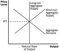
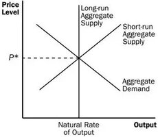
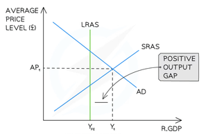
Equilibrium occurs where AD intersects AS. In the short run, equilibrium is at the intersection of AD and SRAS. In the long run, equilibrium is where AD, SRAS, and LRAS all intersect, meaning actual output equals potential output.

Adjustments to Equilibrium

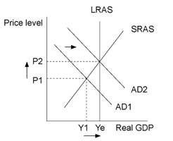
• Increase in AD: Raises both price level and real GDP in the short run; in the long run, only the price level rises as wages and input prices adjust.

• Decrease in AD: Lowers both price level and real GDP in the short run; in the long run, output returns to potential but at a lower price level.

• Increase in SRAS: Raises real GDP and lowers the price level.

• Decrease in SRAS: Causes stagflation (lower GDP and higher prices).

Output Gaps

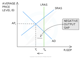
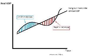
Negative Output Gap (Contractionary/Deflationary Gap)

Occurs when actual output is below potential output. Characterized by higher unemployment, lower inflation, and reduced economic activity.

Positive Output Gap (Expansionary/Inflationary Gap)

Occurs when actual output exceeds potential output. Characterized by low unemployment, rising wages, and upward pressure on prices.

Business Cycle and the AD/AS Model

Explaining the Business Cycle

The AD/AS model illustrates how shifts in aggregate demand and supply drive the business cycle, causing expansions (booms) and contractions (recessions). Demand-side shocks shift AD, while supply-side shocks shift SRAS.

Summary Table: Events and AD/AS Effects

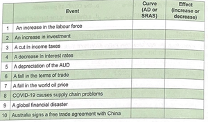
The following table summarizes how various events affect the AD or SRAS curve and whether they increase or decrease aggregate demand or supply.

Event	Curve (AD or SRAS)	Effect (increase or decrease)
An increase in the labour force	SRAS	Increase
An increase in investment	AD	Increase
A cut in income taxes	AD	Increase
A decrease in interest rates	AD	Increase
Depreciation of the AUD	AD	Increase
A fall in the terms of trade	AD	Decrease
A fall in the world oil price	SRAS	Increase
COVID-19 causes supply chain problems	SRAS	Decrease
A global financial disaster	AD	Decrease
Australia signs a free trade agreement with China	AD	Increase

Key Equations

• Aggregate Demand: $AD = C + I + G + (X - M)$

• Output Gap (% of GDP): $\text{Output Gap} = \frac{\text{Actual Output} - \text{Potential Output}}{\text{Potential Output}} \times 100$

Conclusion

The AD/AS model is essential for understanding how economies respond to shocks, policy changes, and structural shifts. It provides a framework for analyzing inflation, unemployment, and economic growth, and is widely used in macroeconomic policy and forecasting.