The AS-AD Model: Aggregate Supply and Aggregate Demand in Macroeconomics

The AS-AD Model

Introduction to the AS-AD Model

The Aggregate Supply-Aggregate Demand (AS-AD) model is a fundamental framework in macroeconomics used to analyze fluctuations in real GDP and the price level. It helps explain economic growth, inflation, and business cycles, and is central to understanding macroeconomic equilibrium and policy effects.

Aggregate Supply

Long-Run Aggregate Supply (LAS)

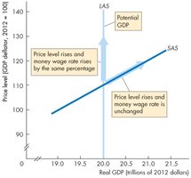
Long-run aggregate supply (LAS) represents the relationship between the quantity of real GDP supplied and the price level when real GDP equals potential GDP. In the long run, money wages are flexible, and the LAS curve is vertical, indicating that changes in the price level do not affect real GDP.

• Potential GDP: The maximum sustainable output of an economy, determined by labor, capital, and technology.

• LAS Curve: Vertical at potential GDP; price level changes matched by money wage changes, so real GDP remains constant.

• Formula: $Y = Y^*$, where $Y$ is real GDP and $Y^*$ is potential GDP.

• Example: If the price level rises and money wages rise by the same percentage, firms supply the same amount of goods.

Short-Run Aggregate Supply (SAS)

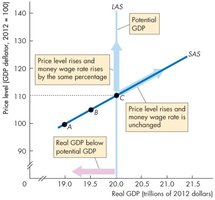
Short-run aggregate supply (SAS) shows the relationship between real GDP supplied and the price level when nominal wages are fixed. The SAS curve is upward sloping, meaning that as the price level rises, firms increase production because real wages fall.

• SAS Curve: Upward sloping; higher price levels increase real GDP supplied.

• Nominal Wages: Fixed in the short run, so real wages decrease as prices rise.

• Example: Firms respond to higher prices by increasing output.

Price Adjustments and Equilibrium

With a given money wage rate, the SAS curve intersects the LAS curve at potential GDP. If the price level falls below equilibrium, the quantity of real GDP supplied decreases along the SAS curve.

• Equilibrium Price Level: Where SAS and LAS intersect.

• Adjustment: Firms reduce output if prices fall below equilibrium.

Changes in Aggregate Supply

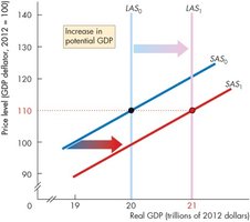
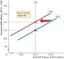
Aggregate supply shifts when factors other than the price level change. These include changes in the money wage rate, potential GDP, labor, capital, and technology.

• Money Wage Rate: Higher wages shift SAS leftward; LAS remains unchanged.

• Potential GDP: Increases shift both LAS and SAS rightward.

• Labor, Capital, Technology: More labor, capital, or technological advances increase potential GDP.

Aggregate Demand

Definition and Determinants

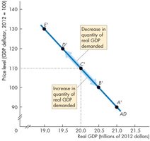
Aggregate demand (AD) is the relationship between the quantity of real GDP demanded and the price level. It is influenced by the price level, expectations, fiscal and monetary policy, and the world economy.

• AD Curve: Downward sloping; higher prices reduce real GDP demanded.

• Determinants: Price level, consumer and business expectations, government policy, global factors.

Reasons for Downward Slope

The AD curve slopes downward due to the wealth effect and substitution effects.

• Wealth Effect: Higher prices reduce purchasing power, lowering consumption.

• Substitution Effects: Intertemporal (future vs. present), international (domestic vs. foreign goods), and home vs. market production.

Factors that Shift the AD Curve

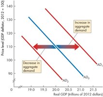
Aggregate demand shifts due to changes in expectations, fiscal and monetary policy, and external economic conditions.

• Expectations: Higher expected income, inflation, or profits increase AD.

• Fiscal Policy: Government spending, tax cuts, and transfers boost AD.

• Monetary Policy: Lower interest rates increase AD.

Macroeconomic Equilibrium

Short-Run Equilibrium

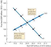
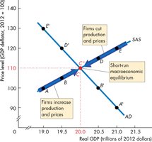
Short-run equilibrium occurs where the AD and SAS curves intersect. At this point, real GDP demanded equals real GDP supplied, but real GDP can be above or below potential GDP.

• Above Potential GDP: Inflationary gap; firms cut production and prices.

• Below Potential GDP: Recessionary gap; firms increase production and prices.

Long-Run Equilibrium

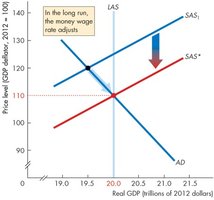
Long-run equilibrium is achieved when real GDP equals potential GDP, at the intersection of the AD and LAS curves. If the economy is below full employment, money wages fall over time, shifting SAS to restore equilibrium.

• Adjustment Mechanism: Money wages adjust to restore full employment.

• Equilibrium Point: Intersection of AD and LAS.

Growth, Inflation, and Business Cycles in the AS-AD Model

Economic Growth

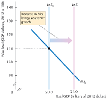
Economic growth occurs when the productive capacity of the economy increases due to population growth, investment, and technological progress. The LAS curve shifts rightward as potential GDP rises.

• Growth Drivers: Labor, capital, technology.

• Effect: LAS and SAS shift right; prices may fall if money supply does not increase.

Inflation

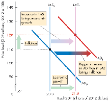
Inflation occurs when aggregate demand increases faster than potential GDP, often due to rapid money supply growth. The AD curve shifts rightward more quickly than LAS, raising the price level.

• Cause: Excessive money supply growth.

• Effect: Higher prices, inflation.

Business Cycles

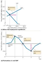
Business cycles are fluctuations in real GDP around potential GDP, caused by changes in aggregate demand and short-run aggregate supply. Money wages do not adjust quickly enough to keep real GDP at potential GDP, resulting in output gaps.

• Inflationary Gap: Real GDP exceeds potential GDP.

• Recessionary Gap: Potential GDP exceeds real GDP.

• No Output Gap: Real GDP equals potential GDP.

Return to Full Employment

Adjustment of Nominal Wages

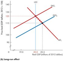
Nominal wages are sticky in the short run but adjust over time to restore full employment. In an inflationary gap, wages rise, shifting SAS leftward. In a recessionary gap, wages fall, shifting SAS rightward.

• Inflationary Gap: Competition for workers raises wages; SAS shifts left.

• Recessionary Gap: High unemployment lowers wages; SAS shifts right.

• Sticky Wages: Wages are slow to adjust, especially downward.

Policy and Shocks in the AS-AD Model

Increasing Aggregate Demand

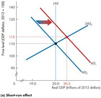
Fiscal and monetary policy are used to stimulate aggregate demand during recessions. An increase in AD shifts the curve rightward, raising production and prices in the short run. Overstimulating demand can lead to inflation.

• Policy Tools: Government spending, tax cuts, lower interest rates.

• Short-Run Effect: Higher output and prices.

Closing an Inflationary Gap

When there is an inflationary gap, the money wage rate rises, shifting SAS leftward. The price level continues to rise, and real GDP decreases until it equals potential GDP.

• Adjustment: Rising wages reduce output, closing the gap.

Negative Supply Shock

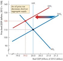
A negative supply shock, such as an oil price increase, shifts the SAS curve leftward. Real GDP decreases and the price level rises, resulting in stagflation—a combination of stagnation and inflation.

• Example: 1970s oil shocks.

• Effect: Lower output, higher prices.

Macroeconomic Schools of Thought

Classical, Monetarist, and Keynesian Views

Macroeconomic schools of thought differ in their views on policy intervention and wage flexibility. Classical and Monetarist economists believe the economy is flexible and self-correcting, while Keynesian economists argue for active policy intervention due to wage and price stickiness.

• Classical/Monetarist: Economy restores full employment on its own; policy intervention unnecessary.

• Keynesian: Economy is sticky; fiscal and monetary policy needed to restore full employment.

• Key Figures: Smith, Ricardo, Mill, Lucas, Prescott (Classical/Monetarist); Keynes, Krugman, Summers (Keynesian).

Additional info: Monetarists emphasize stable money growth, while Keynesians focus on countercyclical policy.