The Classical Model: Full Employment, Labor Market, and Productivity

Study Guide - Smart Notes

Tailored notes based on your materials, expanded with key definitions, examples, and context.

The Classical Model: A Preview

Real and Nominal Variables

The classical model in macroeconomics distinguishes between real variables (such as real GDP, employment, and real wage rate) and nominal variables (such as the price level and nominal wage rate). Real variables describe living standards, while nominal variables reflect changes in dollar values and the value of money.

Real GDP: Measures the value of goods and services produced, adjusted for inflation.
Employment: The number of people working or labor hours employed.
Real Wage Rate: The purchasing power of wages, adjusted for price level.

The classical model determines these real variables at full employment, providing a benchmark for analyzing the actual state of the economy.

Real GDP and Employment

Production Possibilities Frontier (PPF)

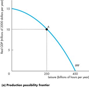
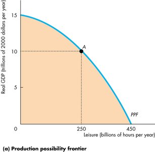
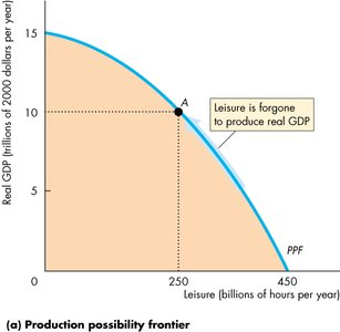
The production possibility frontier (PPF) represents the boundary between combinations of goods and services that can be produced and those that cannot. In macroeconomics, the PPF can illustrate the trade-off between leisure time and real GDP.

Opportunity Cost: The PPF is bowed out, indicating increasing opportunity cost. The most productive labor is used first, and as more labor is employed, it becomes less productive.
Leisure vs. Labor: Forgoing leisure increases labor hours and real GDP.

Example: Moving along the PPF from more leisure to more labor increases real GDP, but at an increasing opportunity cost.

Production possibility frontier between leisure and real GDP PPF showing leisure forgone to produce real GDP

The Production Function

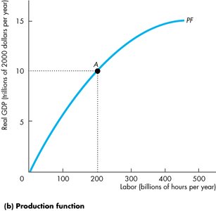
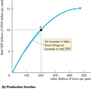
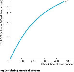
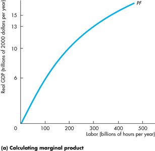
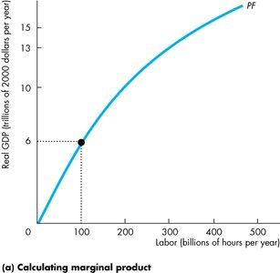
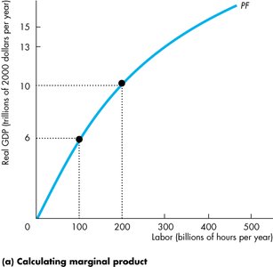
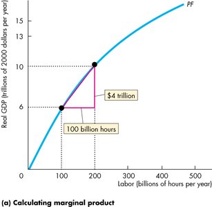
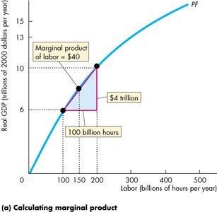
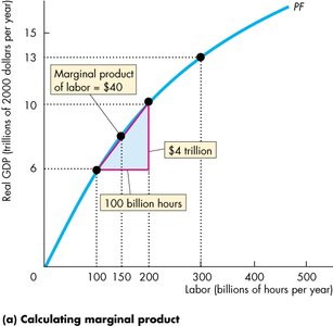
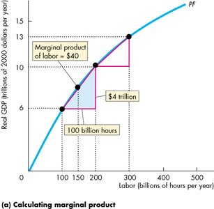
The production function shows the relationship between real GDP and the quantity of labor employed, holding other factors constant. It is the mirror image of the leisure-real GDP PPF.

Increasing Labor: More labor hours increase real GDP, but at a diminishing rate due to decreasing productivity.

Production function: real GDP vs. labor hours Production function: increase in labor hours increases real GDP

The Labor Market and Potential GDP

Demand for Labor

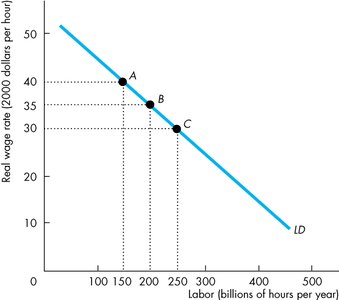
The demand for labor is the relationship between the quantity of labor firms want to hire and the real wage rate. The real wage rate is calculated as:

Formula:
Firms hire labor based on the real wage rate, not the nominal wage rate.

Labor demand curve: real wage rate vs. labor hours

Marginal Product of Labor

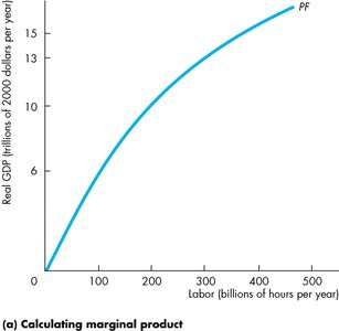
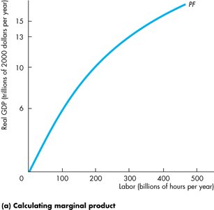
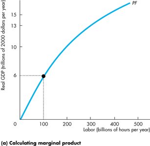
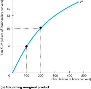
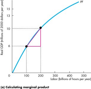
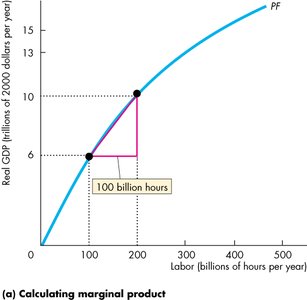
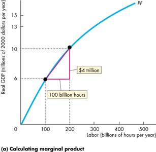
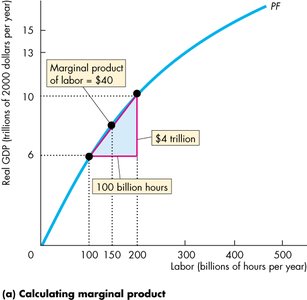
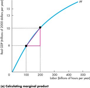
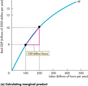
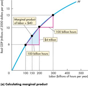
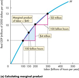
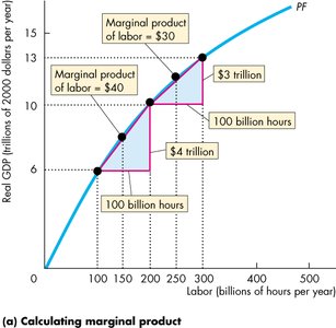
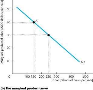
The marginal product of labor is the additional real GDP produced by an extra hour of labor, holding other inputs constant. It follows the law of diminishing returns: as labor increases, marginal product decreases if capital and technology are unchanged.

Formula:
Firms hire labor up to the point where the marginal product equals the real wage rate.

Production function for calculating marginal product Marginal product calculation and curve Marginal product: $4 trillion increase for 100 billion hours Marginal product: $40 per hour Marginal product: $3 trillion for 100 billion hours Marginal product: $30 per hour for 100 billion hours Marginal product curve: $40 and $30 per hour

Supply of Labor

The supply of labor is the relationship between the quantity of labor households are willing to supply and the real wage rate. As the real wage rate increases, labor supply increases due to higher hours per person and increased labor force participation.

Opportunity Cost Effect: Higher real wage rates increase the opportunity cost of not working, encouraging more labor supply.
Income Effect: Higher real wage rates also increase income, which can increase demand for leisure, but the opportunity cost effect usually dominates.

Labor force participation rises with higher real wage rates, but the response is relatively small, making the labor supply curve steep.

Labor Market Equilibrium and Potential GDP

The labor market reaches equilibrium when the quantity of labor demanded equals the quantity supplied. This equilibrium determines the full-employment real wage rate and the potential GDP.

Potential GDP: The level of real GDP at full employment.

Unemployment at Full Employment

Natural Rate of Unemployment

Even at full employment, some unemployment exists, known as the natural rate of unemployment. It arises from:

Job Search: Workers searching for acceptable jobs.
Job Rationing: Wages set above equilibrium, causing excess labor supply.

Job Search

Job search unemployment fluctuates due to demographic changes, unemployment compensation, and structural changes in the economy.

Demographic Change: Younger workers increase frictional unemployment.
Unemployment Compensation: More generous benefits increase search duration.
Structural Change: Technological advances shift jobs between industries.

Job Rationing

Job rationing occurs when wages are set above equilibrium, either through efficiency wages or minimum wages.

Efficiency Wage: Firms pay above equilibrium to attract productive workers and reduce turnover.
Minimum Wage: Legal wage floor; if set above equilibrium, increases unemployment.

Investment, Saving, and the Interest Rate

Investment and Capital

Capital stock is the total amount of plant, equipment, buildings, and inventories. Gross investment is the purchase of new capital, while net investment is gross investment minus depreciation.

Investment Decisions

Expected Profit Rate: Higher expected profits increase investment.
Real Interest Rate: Higher real interest rates decrease investment, as they represent the opportunity cost of funds.

Investment Demand Curve

The investment demand curve shows the relationship between planned investment and the real interest rate. It slopes downward: lower real interest rates increase investment.

Saving

Investment is financed by national saving and borrowing. Saving is current income minus current expenditure.

Personal Saving: Disposable income minus consumption.
Business Saving: Retained profits and pension fund additions.
Government Saving: Budget surplus.
National Saving: Sum of private and government saving.

Factors Influencing Saving

Real Interest Rate: Higher rates increase saving.
Disposable Income: Higher income increases saving.
Wealth: Greater wealth decreases saving.
Expected Future Income: Higher expected income decreases current saving.

Saving Supply Curve

The saving supply curve shows the relationship between saving and the real interest rate. It slopes upward: higher real interest rates increase saving.

Determining the Real Interest Rate

The equilibrium real interest rate is determined by the intersection of the investment demand curve and the saving supply curve. At equilibrium, there is neither a shortage nor surplus of saving.

The Dynamic Classical Model

Changes in Productivity

Labor productivity is real GDP per hour of labor. It is influenced by:

Physical Capital: More capital increases productivity.
Human Capital: Education and training increase productivity.
Technology: Advances increase productivity.

Shifts in the Production Function

Any factor that increases labor productivity shifts the production function upward, increasing real GDP at each labor hour level.

Population and Labor Productivity

Population Increase: Increases labor supply, lowers real wage rate, increases equilibrium labor, and raises potential GDP, but decreases potential GDP per hour.
Labor Productivity Increase: Shifts production function upward, increases demand for labor, real wage rate, labor quantity, and potential GDP.

Example: If population rises, potential GDP increases, but GDP per hour may fall. If productivity rises, both potential GDP and GDP per hour increase.

Additional info: The classical model provides a foundation for understanding full employment, labor market dynamics, and the determinants of productivity and growth in macroeconomics.