The Consumption-Savings Decision in Macroeconomics

Consumption-Savings Decision

Introduction to Consumption and Savings

The consumption-savings decision is a central topic in macroeconomics, focusing on how households allocate income between current consumption and saving for future consumption. This decision is influenced by income, interest rates, and fiscal policy, and is foundational for understanding aggregate demand and long-term economic growth.

• Consumption (C): The aggregate quantity of goods and services households wish to consume.

• Saving (S): The portion of income not consumed, which can be used for future consumption or investment.

• Closed Economy: Assumes no international borrowing or lending (Net Factor Payments, NFP = 0).

Key Equation: The national income identity in a closed economy is $Y = C + I + G$.

Definitions and Notation

• Desired Consumption (C^d): The amount households want to consume given their income and other factors.

• Desired Saving (S^d): The level of national saving when aggregate consumption equals desired consumption.

• Private Saving (S^d_p): The portion of saving done by households and firms.

• Government Saving (S^g): The portion of saving done by the government.

Saving Equation:

$S^d = S^d_p + S^g = Y - C^d - G$

Intertemporal Choice: The Two-Period Model

Basic Structure

The two-period model simplifies the consumption-savings decision by considering only two periods: today (period 1) and the future (period 2). Households choose how much to consume and save in each period to maximize their utility.

• Perfect Capital Markets: Households can borrow or lend at the same real interest rate, r, without constraints.

• Consumption Smoothing: Households prefer a stable consumption path over time, adjusting saving and borrowing to achieve this.

Indifference Curves and Utility

Households' preferences are represented by indifference curves, which show combinations of current and future consumption that yield the same utility level.

• Indifference Curve: $U(C_1, C_2) = \bar{U}$, where $C_1$ is current consumption and $C_2$ is future consumption.

• The curve is negatively sloped: to maintain the same utility, an increase in $C_1$ must be offset by a decrease in $C_2$.

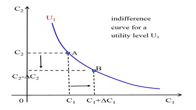
Figure: The indifference curve at a given utility level $U_1$

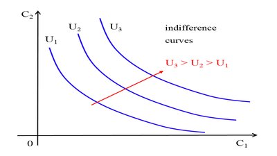
Figure: Indifference curves at different utility levels. Higher curves represent higher utility.

Budget Constraints

The household faces budget constraints in both periods, linking consumption, saving, and income.

• Period 1 (Today): $C_1 + S_p = V + Y_1$

• Period 2 (Future): $C_2 = (1 + r) S_p + Y_2$

• Intertemporal Budget Constraint: Combining both periods gives:

$C_1 + \frac{C_2}{1 + r} = V + Y_1 + \frac{Y_2}{1 + r} \equiv W$

where $W$ is the present value of wealth (initial assets plus the present value of income).

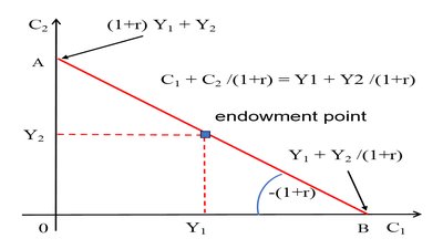
Figure: The intertemporal budget constraint. The slope is $-(1 + r)$, representing the relative price of current to future consumption.

Optimal Consumption Choices: Savers and Borrowers

Households choose the optimal combination of $C_1$ and $C_2$ where the highest indifference curve is tangent to the budget constraint.

• Saver: Consumes less than income in period 1, saves the rest for period 2.

• Borrower: Consumes more than income in period 1 by borrowing against future income.

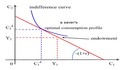
Figure: A saver’s optimal intertemporal choice.

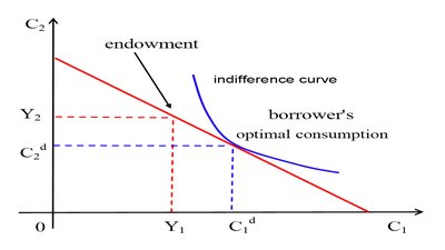
Figure: A borrower’s optimal intertemporal choice.

Effects of Changes in Income and Interest Rates

Impact of Current Income ($Y_1$)

An increase in current income shifts the budget constraint outward, allowing for higher consumption in both periods if consumption is a normal good.

• The slope of the budget constraint remains unchanged; the shift is parallel.

• Both $C_1$ and $C_2$ typically increase, but not by the full amount of the income increase due to consumption smoothing.

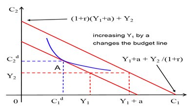
Figure: An increase in $Y_1$ shifts the budget line outward.

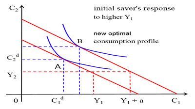
Figure: An initial saver’s response to higher $Y_1$.

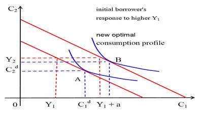
Figure: An initial borrower’s response to higher $Y_1$.

Marginal Propensity to Consume (MPC)

The marginal propensity to consume (MPC) measures the fraction of an additional dollar of income that is consumed in the current period.

• Formula: $MPC = \frac{\Delta C_1}{\Delta Y_1}$

• Typically, $MPC < 1$ because some of the additional income is saved for future consumption.

Impact of Future Income ($Y_2$)

An increase in expected future income raises the present value of wealth, shifting the budget constraint outward and increasing current consumption. However, since current income is unchanged, private saving falls.

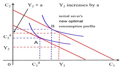
Figure: An initial saver’s response to higher $Y_2$.

Impact of the Real Interest Rate (r)

An increase in the real interest rate changes the slope of the budget constraint, making future consumption relatively cheaper compared to current consumption. This has both substitution and income effects:

• Substitution Effect: Higher r encourages saving (reduces $C_1$, increases $C_2$).

• Income Effect: For savers, higher r increases future income, potentially raising $C_1$ and $C_2$. For borrowers, higher r increases the cost of borrowing, reducing $C_1$ and $C_2$.

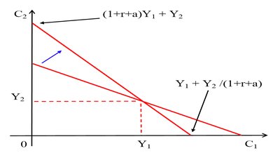
Figure: An increase in r rotates the budget line (relative price change).

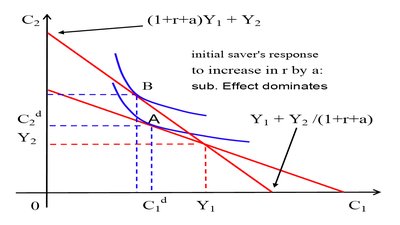
Figure: Initial saver’s response when the substitution effect dominates.

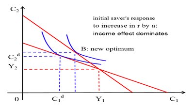
Figure: Initial saver’s response when the income effect dominates.

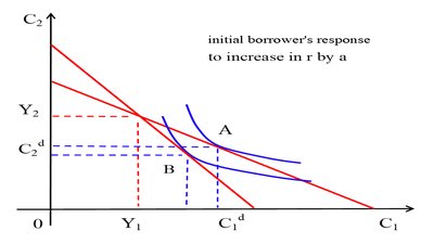
Figure: Initial borrower’s response to a higher r.

Summary Table: Effects of an Increase in r

	Saver	Borrower
Substitution Effect	$C^d_1 \downarrow$, $S^d_p \uparrow$	$C^d_1 \downarrow$, $S^d_p \uparrow$
Income Effect	$C^d_1 \uparrow$, $S^d_p \downarrow$	$C^d_1 \downarrow$, $S^d_p \uparrow$
Overall	Ambiguous	$C^d_1 \downarrow$, $S^d_p \uparrow$

Empirical Evidence: An increase in r generally reduces current consumption and increases saving, but the effect is not very strong.

Conclusion

The consumption-savings decision is a cornerstone of macroeconomic analysis, linking individual behavior to aggregate outcomes. Understanding how households respond to changes in income and interest rates is essential for predicting the effects of fiscal and monetary policy on the economy.