The IS-LM Model: Goods and Financial Markets in Macroeconomics

Goods and Financial Markets: The IS-LM Model

The Goods Market and the IS Relation

The IS-LM model integrates the goods market and the financial market to analyze equilibrium output and interest rates in the economy. The IS relation describes equilibrium in the goods market, where investment depends on both output (income) and the interest rate.

• Investment Function: Investment is a function of output and the interest rate: $I = I(Y, i)$

• Goods Market Equilibrium: The equilibrium condition is: $Y = C(Y - T) + I(Y, i) + G$

• IS Curve: The IS curve shows combinations of output and interest rates where the goods market is in equilibrium. It is downward sloping because higher interest rates reduce investment and thus output.

• Shifts in the IS Curve: Changes in fiscal policy (e.g., taxes or government spending) shift the IS curve. An increase in taxes shifts the IS curve to the left, reducing equilibrium output.

Example:

An increase in taxes reduces disposable income, leading to lower consumption and shifting the IS curve left.

Financial Markets and the LM Relation

The LM relation describes equilibrium in the financial market, where the real money supply equals real money demand. The central bank can set the interest rate by adjusting the money supply.

• Money Market Equilibrium: $M = YL(i)$

• Real Money Balances: $\frac{M}{P} = YL(i)$

• LM Curve: The LM curve is typically horizontal when the central bank targets the interest rate, representing equilibrium in financial markets.

Example:

If the central bank lowers the interest rate, it increases the money supply, shifting the LM curve down.

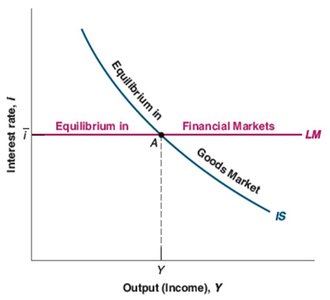
Putting the IS and LM Relations Together

The intersection of the IS and LM curves determines the equilibrium output and interest rate in the economy. Only at this intersection are both goods and financial markets in equilibrium.

• Fiscal Policy: Changes in government spending (G) or taxes (T) shift the IS curve.

• Monetary Policy: Changes in the interest rate (i) or money supply (M) shift the LM curve.

• Policy Analysis Steps: 1. Identify which curve shifts. 2. Determine effects on equilibrium output and interest rate. 3. Describe the effects.

Example:

A fiscal expansion (increase in G-T) shifts the IS curve right, increasing output. A monetary expansion (increase in M) shifts the LM curve down, also increasing output.

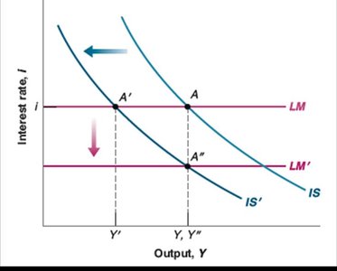
Using a Policy Mix

A combination of fiscal and monetary policies can be used to address economic recessions or to reduce deficits without causing a recession. For example, fiscal consolidation (reducing G-T) can be offset by monetary expansion (lowering i).

Example:

During a recession, both fiscal and monetary expansion can be used to boost output.

Case Study: The US Recession of 2001

The US recession of 2001 was triggered by a sharp decline in investment demand. Macroeconomic policy responses included tax cuts and increased government spending, as well as a reduction in the federal funds rate by the Federal Reserve.

• Growth Rate: Real GDP growth declined during the recession period.

• Federal Funds Rate: The Fed cut the rate from 6.5% to 2% to stimulate the economy.

• Government Revenues and Spending: Tax cuts and increased spending led to changes in government revenues and expenditures as ratios to GDP.

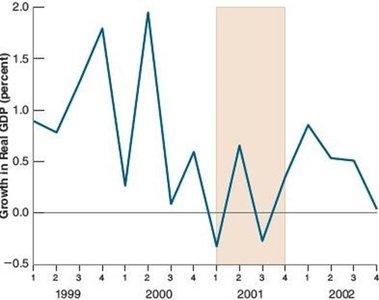
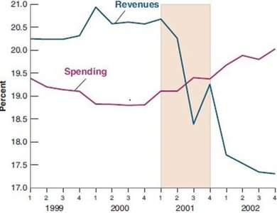
How Does the IS-LM Model Fit the Facts?

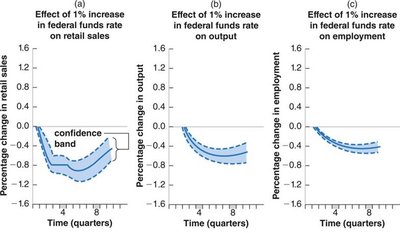
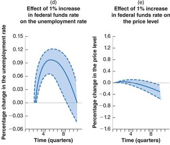
The IS-LM model provides a framework for understanding the effects of monetary and fiscal policy on output and employment. However, real-world adjustments take time due to lags in consumer and firm responses.

• Short-Run Effects: An increase in the federal funds rate leads to decreases in sales, output, and employment, and an increase in unemployment, with little effect on the price level in the short run.

• Empirical Evidence: Studies show that monetary policy shocks have predictable effects on macroeconomic variables.

Additional info:

The IS-LM model is a foundational tool in macroeconomics for analyzing the interplay between fiscal and monetary policy and their effects on aggregate output and interest rates. It is especially useful for short-run analysis, though it must be supplemented with dynamic considerations for real-world applications.