The Simplest Short-Run Macro Model: Consumption, Investment, and Aggregate Expenditure

6a Desired Consumption Expenditure

Autonomous and Induced Expenditures

In macroeconomics, expenditures are classified based on their dependence on national income (Y). Understanding this distinction is crucial for analyzing how changes in income affect overall spending in the economy.

• Autonomous expenditures: These do not depend on the level of national income. Examples include basic consumption needs or fixed investments.

• Induced expenditures: These do depend on the level of national income. As income rises, induced expenditures increase.

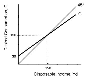
Disposable Income and the Consumption Function

Disposable income (YD) is the income available to households after taxes:

$Y_D = Y - T$

The consumption function models desired consumption as a linear function of disposable income:

$C = a + bY_D$

• a = autonomous consumption (consumption when income is zero)

• b = marginal propensity to consume (MPC)

Example: $C = 30 + 0.8Y_D$

Marginal Propensity to Consume (MPC)

The MPC is the proportion of additional disposable income that consumers spend:

$MPC = \frac{\Delta C}{\Delta Y_D}$

• The MPC is the slope of the consumption function.

Movements and Shifts in the Consumption Function

• Movement along the function: Caused by changes in disposable income.

• Shifts of the function: Caused by changes in wealth, interest rates, or expectations.

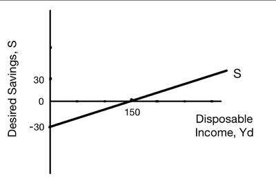
Savings and the Marginal Propensity to Save (MPS)

Disposable income not spent is saved:

$S = Y_D - C$

The marginal propensity to save (MPS) is:

$MPS = \frac{\Delta S}{\Delta Y_D}$

6b Desired Investment Expenditure

Autonomous Nature of Investment

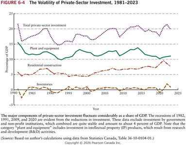
Investment is the most volatile component of GDP and is typically modeled as autonomous—independent of current national income. This is because investment decisions are based on long-term planning and expectations.

• Investment is strongly associated with short-run economic fluctuations.

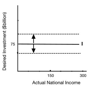
The Investment Function

The investment function is usually depicted as a horizontal line, indicating that desired investment does not change with current income:

$I = I_0$

• Shifts in the investment function can be caused by:

  • Changes in the real interest rate (opportunity cost of investment)

  • Changes in the level of sales (affecting desired inventory levels and capacity utilization)

  • Business confidence (forward-looking expectations)

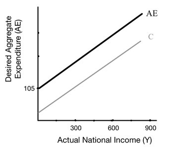
6c The Aggregate Expenditure Function

Definition and Construction

The aggregate expenditure (AE) function relates total desired spending in the economy to actual national income (Y). In the simplest model (no government, no trade, constant prices):

$AE = C + I$

Where $C$ is a function of $Y$ (not $Y_D$ in this simplified case), and $I$ is autonomous.

• Example: $C = 30 + 0.8Y$, $I = 75$

Marginal Propensity to Spend (z)

The marginal propensity to spend (z) is the extra desired AE induced by an additional $1 of national income:

$z = \frac{dAE}{dY}$

• In this simple model (no taxes), $z = MPC$

6d Equilibrium National Income

Determination of Equilibrium

Equilibrium national income occurs where desired aggregate expenditure equals actual national income:

$AE = Y$

• If $AE > Y$, inventories fall and firms increase output.

• If $AE < Y$, inventories rise and firms reduce output.

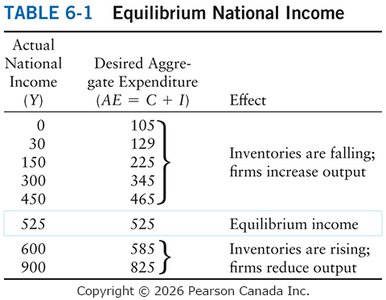
Table: Equilibrium National Income

The following table illustrates how equilibrium is achieved:

Actual National Income (Y)	Desired Aggregate Expenditure (AE = C + I)	Effect
0	105	Inventories are falling; firms increase output
30	129	Inventories are falling; firms increase output
150	225	Inventories are falling; firms increase output
300	345	Inventories are falling; firms increase output
450	465	Inventories are falling; firms increase output
525	525	Equilibrium income
600	585	Inventories are rising; firms reduce output
900	825	Inventories are rising; firms reduce output

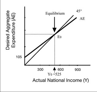
Graphical Representation of Equilibrium

Equilibrium is found where the AE curve intersects the 45-degree line (where AE = Y):

Example: $AE = 105 + 0.8Y$ Solving for equilibrium: $Y_0 = 525$

6e The Simple Multiplier

Definition and Calculation

The simple multiplier (SM) measures the change in equilibrium national income resulting from a change in autonomous expenditure:

$SM = \frac{\Delta Y}{\Delta A} = \frac{1}{1 - z}$

• The larger the marginal propensity to spend (z), the larger the multiplier.

• A change in autonomous expenditure causes a parallel shift in the AE curve, leading to a multiplied change in equilibrium income.

Example: If $C = 30 + 0.75Y$ and $I$ increases by 10, calculate the change in $Y$ using the multiplier formula.

Additional info: The multiplier effect is a central concept in Keynesian economics, illustrating how initial changes in spending can have amplified effects on total output and income.