Chapter 1: Representing Motion – Physics with Algebra Study Notes

Chapter 1: Representing Motion

Introduction to Motion

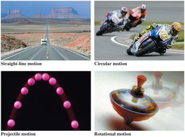
Motion is a fundamental concept in physics, describing the change of an object’s position or orientation with time. The path along which an object moves is called its trajectory. Understanding motion is essential for analyzing and predicting the behavior of objects in the physical world.

• Types of Motion: Motion can be classified into several types, including straight-line (linear) motion, circular motion, projectile motion, and rotational motion.

• Trajectory: The specific path taken by an object as it moves.

Section 1.1: Motion – A First Look

Making a Motion Diagram

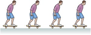
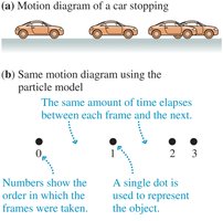
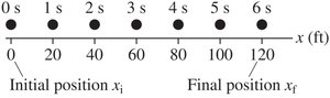
Motion diagrams are visual tools that represent the position of an object at successive time intervals. They help us analyze how an object moves over time, whether at constant speed, speeding up, or slowing down.

• Constant Speed: Equal spacing between positions indicates uniform motion.

• Speeding Up: Increasing spacing between positions shows acceleration.

• Slowing Down: Decreasing spacing between positions shows deceleration.

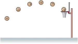
Motion in two dimensions can involve changes in both speed and direction, such as a basketball following a curved path toward a hoop.

Section 1.2: Models and Modeling

Models in Physics

Models are simplified representations of physical systems that capture essential features while ignoring unnecessary details. They are crucial for understanding and predicting physical phenomena.

• Descriptive Models: Describe properties in the simplest terms possible.

• Explanatory Models: Use laws of physics to predict outcomes.

• Particle Model: Treats a moving object as if all its mass is concentrated at a single point, simplifying analysis.

Section 1.3: Position and Time – Putting Numbers on Nature

Position and Coordinate Systems

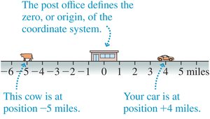
To specify an object’s position, we use a reference point (origin), a distance from the origin, and a direction. A coordinate system consists of an origin and an axis marked in positive and negative directions.

• Coordinate: Symbol representing a position along an axis (e.g., x, y).

Time

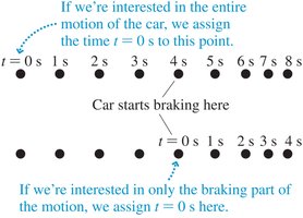
Each position in a motion diagram is associated with a specific time, denoted by the symbol t. Time intervals are essential for quantifying motion.

Changes in Position and Displacement

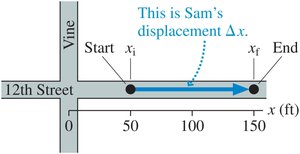
Displacement is the difference between an object’s final and initial positions. It is a vector quantity, meaning it has both magnitude and direction.

• Displacement formula: $\Delta x = x_f - x_i$

Change in Time (Time Interval)

The time interval is the difference between the final and initial times as an object moves from one position to another. It is always positive.

• Time interval formula: $\Delta t = t_f - t_i$

Example: How Long a Ride?

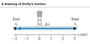
Emily rides her bicycle from 3 miles east to 2 miles west of a water tower in half an hour. Her displacement is calculated as:

• $\Delta x = x_f - x_i = (-2) - (3) = -5$ miles (westward)

Section 1.4: Velocity

Velocity and Speed

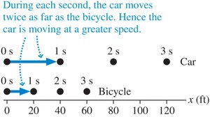
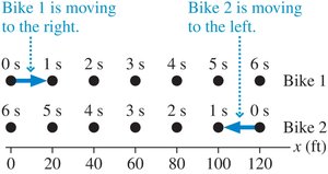
Speed is a scalar quantity that measures how fast an object moves, while velocity is a vector that includes both speed and direction. Uniform motion refers to motion at a constant speed in a straight line.

• Average velocity: $v_{avg} = \frac{\Delta x}{\Delta t}$

Section 1.5: Significant Figures, Scientific Notation, and Units

Measurements and Significant Figures

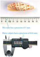
Measurements are limited by the precision of the measuring instrument. Significant figures reflect the certainty of a measurement.

• All non-zero digits are significant.

• Zeros between non-zero digits are significant.

• Leading zeros are not significant.

• Trailing zeros after a decimal point are significant.

• Trailing zeros without a decimal point may or may not be significant; use scientific notation to clarify.

Using Significant Figures in Calculations

• Multiplication/Division: Round to the fewest significant figures.

• Addition/Subtraction: Round to the fewest decimal places.

• Exact numbers: Do not affect significant figures.

Scientific Notation

Scientific notation expresses very large or small numbers in the form $a \times 10^n$, where $1 \leq a < 10$ and $n$ is an integer.

• Example: $5,200 = 5.2 \times 10^3$

• Example: $0.00089 = 8.9 \times 10^{-4}$

Rules for Operations Using Scientific Notation

• Multiplication: Multiply the numbers, add the exponents.

• Division: Divide the numbers, subtract the exponents.

Units and Unit Conversion

Units are standard quantities used to specify measurements. The International System of Units (SI) is the standard system in science.

• Base units: meter (m), kilogram (kg), second (s)

• Derived units: meters per second (m/s), newton (N)

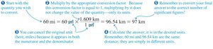
Unit conversions use conversion factors to change from one unit to another.

Estimation and Order-of-Magnitude

An order-of-magnitude estimate is a rough calculation, usually accurate to within a factor of 10, and is indicated by the symbol "~".

Section 1.6: Vectors and Motion – A First Look

Scalars and Vectors

Scalars are quantities with only magnitude (e.g., length, mass, time). Vectors have both magnitude and direction (e.g., displacement, velocity). Vectors are represented graphically by arrows.

Adding and Subtracting Vectors

Vectors can be added or subtracted graphically or by breaking them into components.

• Graphical Addition: Place vectors head-to-tail; the resultant vector is drawn from the tail of the first to the head of the last.

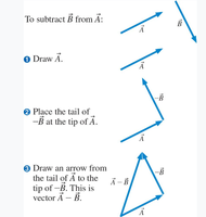
• Graphical Subtraction: Reverse the direction of the vector to be subtracted, then add as usual.

Example: How Far Away Is Anna?

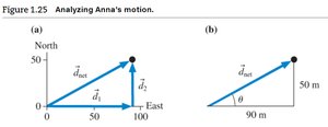
Anna walks 90 m east, then 50 m north. Her displacement is the straight-line distance from her starting point to her final position, found using the Pythagorean theorem:

• $d_{net} = \sqrt{(90)^2 + (50)^2} = \sqrt{8100 + 2500} = \sqrt{10600} \approx 103$ m

Vectors and Trigonometry

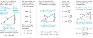
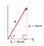
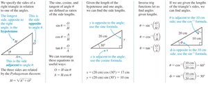
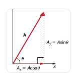
Trigonometry is used to resolve vectors into components. For a vector of magnitude $A$ at an angle $\theta$ from the horizontal:

• Horizontal component: $A_x = A \cos(\theta)$

• Vertical component: $A_y = A \sin(\theta)$

Example: A hiker walks 5 km at a 60° angle from east.

• Eastward component: $5 \cos(60°) = 2.5$ km

• Northward component: $5 \sin(60°) \approx 4.3$ km