1D Kinematics: Describing Motion in One Dimension

1D Kinematics: Describing Motion in One Dimension

Reference Frames & Displacement

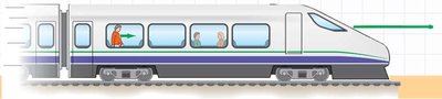
To describe the motion of an object, we must specify its position relative to a chosen reference frame. This involves selecting an origin, a positive direction, and a coordinate axis. The concept of displacement distinguishes between the total path traveled and the straight-line change in position.

• Reference Frame: The perspective from which position and motion are measured. Choosing a reference frame involves selecting an origin and a direction for positive values.

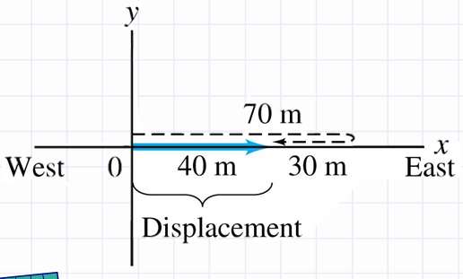
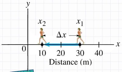
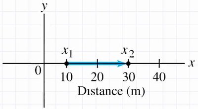
• Displacement (\( \Delta x \)): The straight-line change in position from the initial point (\( x_1 \)) to the final point (\( x_2 \)). It is a vector and can be positive or negative, indicating direction.

• Distance: The total length of the path traveled, regardless of direction. It is always positive and is a scalar quantity.

• Formula: $\Delta x = x_2 - x_1$

• Example: If a person walks from 30 m to 10 m on the x-axis, their displacement is $\Delta x = 10\,\text{m} - 30\,\text{m} = -20\,\text{m}$ (to the left).

Speed & Velocity

Kinematics describes how objects move, not why. Speed and velocity are fundamental concepts for quantifying motion.

• Speed: The rate at which distance is covered. It is a scalar and always positive.

• Average Speed: $v_{\text{avg}} = \frac{d}{t}$, where d is total distance and t is total time.

• Instantaneous Speed: The speed at a specific instant in time (what a speedometer reads).

• Velocity: The rate of change of displacement. It is a vector and can be positive, negative, or zero.

• Average Velocity: $\vec{v}_{\text{avg}} = \frac{\Delta x}{\Delta t}$

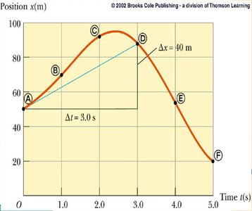
• Instantaneous Velocity: The velocity at a specific instant, given by the slope of the tangent to a position-time graph at that point.

• Example: If you travel 100 miles in 2 hours, your average speed is $50\,\text{mph}$, but your instantaneous speed may vary during the trip.

Position-Time Graphs and Velocity

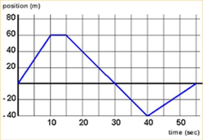
Position-time graphs visually represent how an object's position changes over time. The slope of the graph at any point gives the velocity.

• Positive Slope: Positive velocity (moving in the positive direction).

• Negative Slope: Negative velocity (moving in the negative direction).

• Zero Slope: Zero velocity (object is at rest).

• Steeper Slope: Greater speed.

• Average Velocity from Graph: Slope of the secant line between two points.

• Instantaneous Velocity from Graph: Slope of the tangent line at a specific point.

Acceleration

Acceleration is the rate at which velocity changes. It can result from changes in speed, direction, or both. Acceleration is a vector and can be positive or negative depending on the chosen direction.

• Definition: $a = \frac{\Delta v}{\Delta t}$

• Units: meters per second squared (m/s2).

• Acceleration occurs when:

  • Speed increases (velocity and acceleration in the same direction).

  • Speed decreases (velocity and acceleration in opposite directions).

  • Direction changes (even if speed is constant).

• Examples:

  • A car speeding up from a stoplight (positive acceleration).

  • An airplane slowing to a stop (negative acceleration).

  • An object moving in a circle (changing direction, so accelerating).

Velocity-Time Graphs and Acceleration

Velocity-time graphs show how velocity changes over time. The slope of the graph gives the acceleration.

• Positive Slope: Positive acceleration.

• Negative Slope: Negative acceleration.

• Zero Slope: Zero acceleration (constant velocity).

• Steeper Slope: Greater magnitude of acceleration.

• Formula: $a = \frac{\Delta v}{\Delta t}$

Constant Acceleration Equations

When acceleration is constant, a set of equations (kinematic equations) can be used to predict an object's position and velocity at any time. These equations are derived from the definitions of velocity and acceleration.

• $v = v_0 + at$

• $x = x_0 + v_0 t + \frac{1}{2} a t^2$

• $v^2 = v_0^2 + 2a\Delta x$

• Where:

  • $v_0$ = initial velocity

  • $v$ = final velocity

  • $a$ = acceleration

  • $x_0$ = initial position

  • $x$ = final position

  • $t$ = time

  • $\Delta x = x - x_0$

Problem-Solving Strategy for Constant Acceleration

1. Choose a coordinate system (define positive direction).

2. List known and unknown quantities.

3. Identify what you are solving for.

4. Choose the appropriate equation(s).

5. Solve algebraically, then substitute numbers.

6. Check signs, units, and reasonableness of your answer.

Free-Fall: A Special Case of Constant Acceleration

Free-fall refers to motion under the influence of gravity alone, with air resistance neglected. The acceleration due to gravity near Earth's surface is $g \approx -9.80\,\text{m/s}^2$ (downward, if upward is positive).

• Free-fall equations: Same as constant acceleration, but use $y$ for vertical displacement and $g$ for acceleration.

• Key equations:

  • $v = v_0 + gt$

  • $y = y_0 + v_0 t + \frac{1}{2} g t^2$

  • $v^2 = v_0^2 + 2g\Delta y$

• Sign conventions: Upward is usually positive; downward is negative.

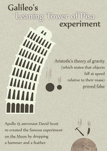
• Galileo's Experiment: Demonstrated that all objects fall at the same rate regardless of mass (neglecting air resistance).

Summary Table: Kinematic Quantities

Quantity	Definition	Vector/Scalar	Key Equation
Displacement (\(\Delta x\))	Change in position	Vector	$\Delta x = x_2 - x_1$
Distance	Total path length	Scalar	Sum of all path segments
Velocity (\(v\))	Rate of change of displacement	Vector	$v = \frac{\Delta x}{\Delta t}$
Speed	Rate of change of distance	Scalar	$v = \frac{d}{t}$
Acceleration (\(a\))	Rate of change of velocity	Vector	$a = \frac{\Delta v}{\Delta t}$

Key Takeaways

• Motion is always described relative to a reference frame.

• Displacement and velocity are vectors; distance and speed are scalars.

• Acceleration describes changes in velocity (speed or direction).

• Constant acceleration allows use of kinematic equations for prediction.

• Free-fall is a special case of constant acceleration with $a = g$.