Chapter 1: Concepts of Motion – Structured Study Notes

Concepts of Motion

Introduction to Motion

Motion is a fundamental concept in physics, describing the change in position of objects over time. Understanding motion is essential for analyzing physical phenomena and forms the basis for more advanced topics in mechanics.

Types of Motion

There are four basic types of motion commonly encountered in physics:

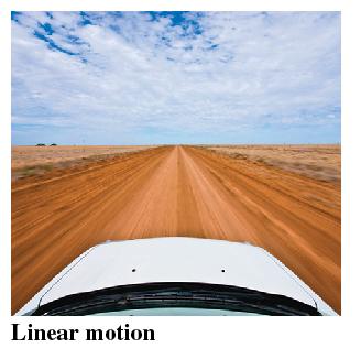
• Linear Motion: Movement along a straight path.

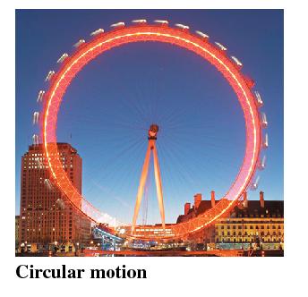
• Circular Motion: Movement along a circular path.

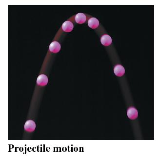
• Projectile Motion: Movement of an object thrown into the air, subject to gravity.

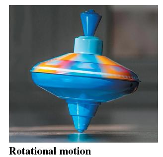
• Rotational Motion: Movement around an axis.

Motion Diagrams

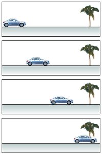
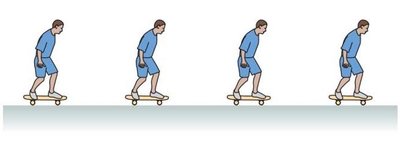
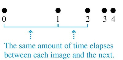
A motion diagram is a visual tool used to represent the positions of an object at successive times. It helps in analyzing the nature of motion, such as whether the object is moving at constant speed, speeding up, or slowing down.

• Each frame in a motion diagram corresponds to a specific instant in time.

• Equally spaced images indicate constant speed.

• Increasing distance between images shows speeding up.

• Decreasing distance between images shows slowing down.

The Particle Model

In many cases, it is useful to model an object as a particle, concentrating all its mass at a single point. This simplifies the analysis of motion, especially when the object's size and shape are not important.

• Each dot in a motion diagram represents the particle's position at a given time.

• The particle model is used for objects like cars, rockets, or dust particles.

Position and Time

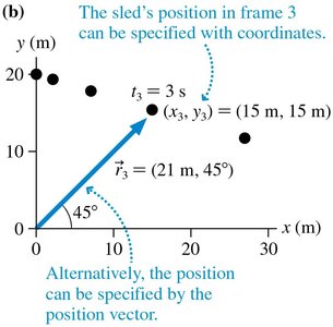
To analyze motion, it is necessary to specify both the position and the time at which the object occupies that position. This is often done using a coordinate system.

• Position is given by coordinates (x, y) or by a position vector \( \vec{r} \).

• Time is measured relative to a chosen origin.

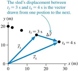
Displacement

Displacement is a vector quantity representing the change in position of an object. It is defined as:

• \( \Delta \vec{r} = \vec{r}_f - \vec{r}_i \)

• Displacement points from the initial position to the final position.

Vector Addition

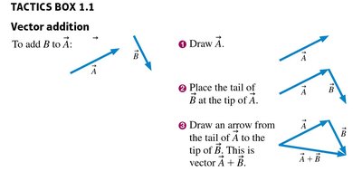
Vectors are added using the tip-to-tail method. This is essential for combining displacements, velocities, and accelerations.

• Draw the first vector.

• Place the tail of the second vector at the tip of the first.

• Draw the resultant vector from the tail of the first to the tip of the second.

Time Interval

The time interval is the difference between two times:

• \( \Delta t = t_f - t_i \)

• All observers agree on the value of \( \Delta t \) and \( \Delta \vec{r} \).

Average Speed and Average Velocity

Average speed is a scalar quantity, while average velocity is a vector:

• Average speed: \( \text{average speed} = \frac{d}{\Delta t} \)

• Average velocity: \( \vec{v}_{\text{avg}} = \frac{\Delta \vec{r}}{\Delta t} \)

Motion Diagrams with Velocity Vectors

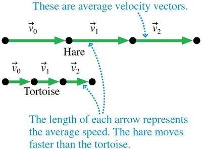
Velocity vectors are drawn connecting the dots in a motion diagram. The direction and length of the vector indicate the direction and magnitude of velocity.

• Velocity vectors are proportional to displacement vectors.

• Label the vectors as \( \vec{v} \).

Linear Acceleration

Acceleration describes the rate of change of velocity:

• \( \Delta \vec{v} = \vec{v}_2 - \vec{v}_1 \)

• Average acceleration: \( a_{\text{avg}} = \frac{\Delta \vec{v}}{\Delta t} \)

Finding the Acceleration Vector

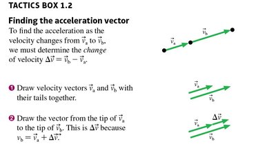
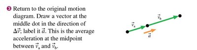
To find the acceleration vector, determine the change in velocity between two points and draw the vector at the midpoint.

• Draw velocity vectors with their tails together.

• Draw the change in velocity vector \( \Delta \vec{v} \).

• Draw the acceleration vector at the midpoint.

Speeding Up or Slowing Down

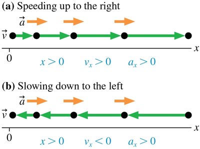
The relationship between velocity and acceleration vectors determines whether an object is speeding up or slowing down:

• If velocity and acceleration point in the same direction, the object speeds up.

• If they point in opposite directions, the object slows down.

• Velocity is constant if acceleration is zero.

Position-versus-Time Graphs

Position-versus-time graphs provide another way to represent motion. The slope of the graph indicates velocity, and changes in slope indicate acceleration.

• Linear segments indicate constant velocity.

• Horizontal segments indicate the object is at rest.

Units and Unit Conversions

Physics uses the SI system of units:

• Time: second (s)

• Length: meter (m)

• Mass: kilogram (kg)

• Prefixes denote powers of ten (e.g., kilo-, milli-, micro-).

Prefix	Power of 10	Abbreviation
giga-	109	G
mega-	106	M
kilo-	103	k
centi-	10-2	c
milli-	10-3	m
micro-	10-6	μ
nano-	10-9	n

Significant Figures

Significant figures indicate the precision of a measurement. Calculations should reflect the least precise input value.

• Report results with the correct number of significant figures.

• Use the "weakest link" rule for calculations.

Orders of Magnitude and Estimating

An order-of-magnitude estimate is a rough calculation, usually accurate to within a factor of ten. It is useful for quick assessments and comparisons.

• Symbol: ~ (less precise than ≈)

• Examples: Length of a football field ~ 100 m; Mass of a textbook ~ 1 kg.

Object	Length (m)
Altitude of jet planes	10,000
Distance across campus	1,000
Length of a football field	100
Length of a classroom	10
Length of your arm	1
Width of a textbook	0.1
Length of a fingernail	0.01

Object	Mass (kg)
Small car	10,000
Large human	100
Medium-size dog	10
Science textbook	1
Apple	0.1
Pencil	0.01
Raisin	0.001

Problem-Solving Strategy

Solving physics problems involves several steps:

1. Model: Simplify the situation using an appropriate model (e.g., particle model).

2. Visualize: Draw pictorial and graphical representations to clarify the problem.

3. Solve: Develop and solve mathematical equations based on the model.

4. Review: Assess the result for reasonableness, units, and significant figures.

Summary

Chapter 1 introduces the essential concepts of motion, including types of motion, motion diagrams, vectors, displacement, velocity, acceleration, units, significant figures, and problem-solving strategies. Mastery of these concepts is foundational for further study in physics with calculus.