Chapter 2: Motion in One Dimension – Structured Study Notes

Motion in One Dimension

Introduction to Linear Motion

Motion in one dimension refers to the movement of objects along a straight line, either horizontally or vertically. This chapter focuses on describing, analyzing, and solving problems related to linear motion using various representations such as graphs, diagrams, and equations.

• Key Kinematic Variables: Position, velocity, and acceleration.

• Representations: Graphical, pictorial, and mathematical.

• Types of Motion: Uniform motion and motion with constant acceleration (including free fall).

Describing Motion

Motion can be described using position, velocity, and acceleration. The position of an object is typically represented along an axis (x for horizontal, y for vertical).

• Position: The location of an object relative to a reference point.

• Velocity: The rate of change of position with respect to time; includes direction.

• Acceleration: The rate of change of velocity with respect to time.

Position-Versus-Time Graphs

Position-versus-time graphs are fundamental tools for analyzing motion. The slope of the graph at any point gives the velocity of the object.

• Steeper Slope: Indicates faster speed.

• Positive Slope: Motion to the right (or up).

• Negative Slope: Motion to the left (or down).

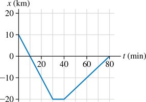
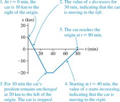
Interpreting Position Graphs

Understanding the motion from a position graph involves identifying intervals of movement, rest, and changes in direction.

• At t = 0, the object starts at a certain position.

• Negative slope indicates movement to the left.

• Flat segments indicate periods of rest.

• Positive slope indicates movement to the right.

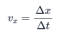
From Position to Velocity

The velocity of an object can be determined from the slope of its position-versus-time graph. The velocity-versus-time graph provides another representation of motion.

• Formula: $v_x = \frac{\Delta x}{\Delta t}$

• Velocity is positive for motion to the right, negative for motion to the left.

From Velocity to Position

The position graph can be deduced from the velocity graph. The area under the velocity-versus-time graph gives the displacement.

• Displacement: Area under the velocity graph during a time interval.

• Sign of Velocity: Indicates direction of motion.

Uniform Motion

Uniform motion is straight-line motion in which equal displacements occur during any successive equal-time intervals. The position-versus-time graph for uniform motion is a straight line.

• Equation: $x = x_0 + v_x t$

• Velocity: Constant throughout the motion.

Instantaneous Velocity

Instantaneous velocity is the velocity of an object at a specific instant. It is found by calculating the slope of the tangent to the position-versus-time curve at that point.

• If the position graph is curved, the instantaneous velocity is the slope of the tangent line.

• Graphical Method: Magnify the segment around the point of interest to approximate the slope.

Acceleration

Acceleration describes how an object's velocity changes over time. It is the slope of the velocity-versus-time graph.

• Definition: $a = \frac{\Delta v}{\Delta t}$

• Positive acceleration: Speeding up in the positive direction.

• Negative acceleration: Slowing down or speeding up in the negative direction.

Motion with Constant Acceleration

When an object moves with constant acceleration, its velocity changes linearly with time, and its position changes as the square of the time interval.

• Velocity Equation: $v = v_0 + a t$

• Position Equation: $x = x_0 + v_0 t + \frac{1}{2} a t^2$

• Displacement Equation: $\Delta x = \frac{v_0 + v}{2} t$

• Velocity-Distance Relation: $v^2 = v_0^2 + 2 a \Delta x$

Free Fall

Free fall is the motion of objects under the influence of gravity only. All objects in free fall have the same acceleration, regardless of their mass.

• Free-Fall Acceleration: $g = 9.8\ \text{m/s}^2$ (downward)

• Use kinematic equations with $a = -g$ for vertical motion.

• At the highest point, velocity is zero; acceleration remains constant.

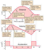
Graphical Summary of Motion

Graphs of position, velocity, and acceleration provide a comprehensive view of an object's motion. Key features include slopes, areas under curves, and points of zero velocity or acceleration.

Problem-Solving Strategy

Solving motion problems involves a systematic approach:

1. Strategize: Identify the type of problem and the relevant equations.

2. Prepare: Draw diagrams, establish coordinate systems, and collect information.

3. Solve: Apply equations and perform calculations.

4. Assess: Check if the solution makes physical sense.

Example Table: Kinematic Equations for Constant Acceleration

Equation	Description
$v = v_0 + a t$	Final velocity after time t
$x = x_0 + v_0 t + \frac{1}{2} a t^2$	Position after time t
$\Delta x = \frac{v_0 + v}{2} t$	Displacement during time t
$v^2 = v_0^2 + 2 a \Delta x$	Velocity as a function of displacement

Applications and Examples

• Train Problem: Ratio reasoning for uniform motion.

• Car Braking: Using constant acceleration equations to find stopping distance.

• Rocket Launch: Calculating velocity and distance using kinematic equations.

• Free Fall: Determining fall time and impact velocity for dropped objects.

Summary

Motion in one dimension is foundational for understanding physics. Mastery of position, velocity, and acceleration, along with their graphical and mathematical representations, is essential for solving real-world problems involving linear motion.