College Physics I: Models, Measurements, Vectors, and Motion Along a Straight Line

Units, Physical Quantities, and Vectors

The Nature of Physics

Physics is the study of the fundamental laws of nature and their interactions. It relies on precise measurements and mathematical models to describe physical phenomena.

Solving Physics Problems

• Identify knowns and unknowns: List all given quantities and what needs to be found.

• Establish a coordinate system: Choose axes and origin for clarity.

• Apply relevant equations: Use mathematical relationships to solve for unknowns.

Standards and Units

• SI Units: The International System of Units (SI) is used for consistency in physics.

• Base units: Meter (m), kilogram (kg), second (s), ampere (A), kelvin (K), mole (mol), candela (cd).

Unit Consistency and Conversions

• Unit consistency: Always check that equations use compatible units.

• Conversions: Use conversion factors to switch between units (e.g., 1 km = 1000 m).

Uncertainty and Significant Figures

• Uncertainty: Every measurement has an associated uncertainty.

• Significant figures: Indicate the precision of a measurement.

Vectors and Vector Addition

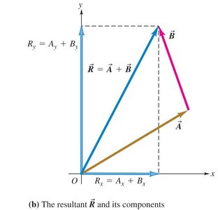
Vectors are quantities with both magnitude and direction, such as displacement, velocity, and force. Vector addition can be performed graphically (tip-to-tail method) or algebraically using components.

• Vector notation: \vec{A} represents a vector.

• Magnitude: The length of the vector.

• Direction: The angle relative to a reference axis.

Components of Vectors

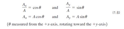
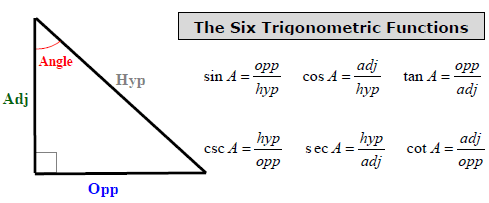
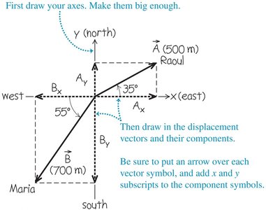
Any vector in two dimensions can be broken down into x and y components using trigonometry:

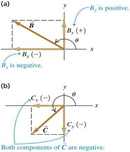
• Component equations: $A_x = A \cos \theta$ $A_y = A \sin \theta$ where $\theta$ is measured from the +x-axis, rotating toward the +y-axis.

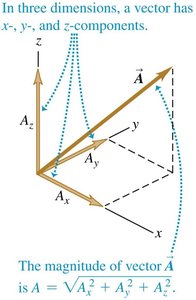
• Magnitude from components: $A = \sqrt{A_x^2 + A_y^2}$

Vector Addition Using Components

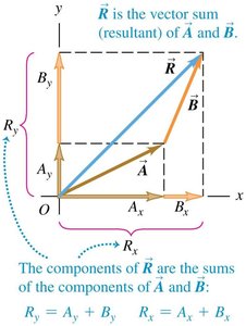
Vectors can be added by summing their respective components:

• $R_x = A_x + B_x$

• $R_y = A_y + B_y$

• Resultant vector: $\vec{R} = \vec{A} + \vec{B}$

Motion Along a Straight Line

Displacement, Time, and Average Velocity

Kinematics is the study of motion. For straight-line motion, displacement, time, and velocity are key concepts.

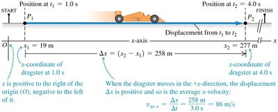
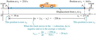
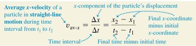
• Displacement: Change in position along the x-axis, $\Delta x = x_2 - x_1$.

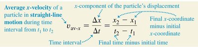
• Average velocity: $v_{\text{av}-x} = \frac{\Delta x}{\Delta t}$

Instantaneous Velocity

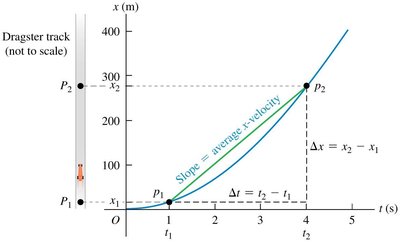
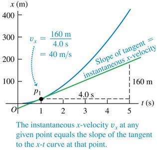
The instantaneous velocity is the velocity at a specific instant, given by the slope of the tangent to the position-time graph.

• $v_x = \frac{dx}{dt}$

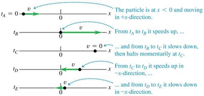
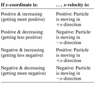
Rules for the Sign of x-Velocity

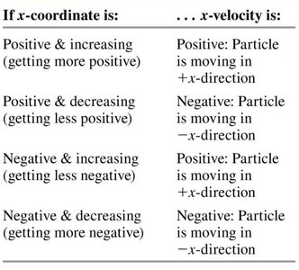
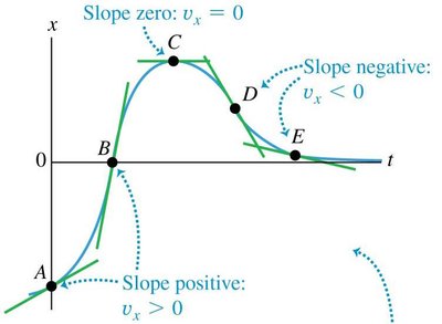
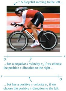
The sign of velocity depends on the direction of motion and the coordinate system.

• Positive velocity: Moving in +x direction

• Negative velocity: Moving in -x direction

Average and Instantaneous Acceleration

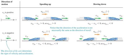
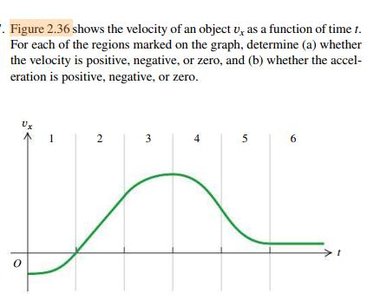
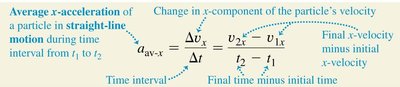
Acceleration describes the rate of change of velocity with time.

• Average acceleration: $a_{\text{av}-x} = \frac{\Delta v_x}{\Delta t}$

• Instantaneous acceleration: $a_x = \frac{dv_x}{dt}$

Approaching Kinematics Problems

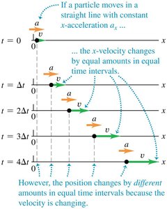
• Draw a motion diagram and determine acceleration vectors.

• Establish a coordinate system and label axes.

• Draw arrows for acceleration between positions.

• Make a table of knowns and unknowns.

• Use kinematic equations to solve.

Motion with Constant Acceleration

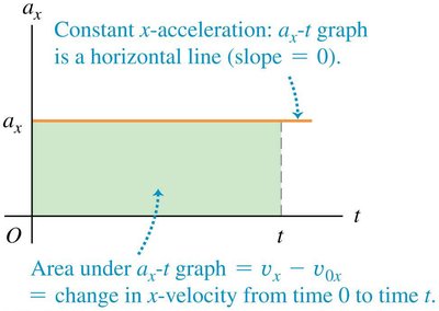
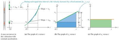
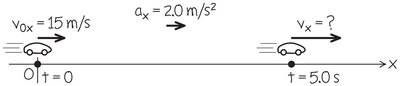
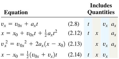
When acceleration is constant, the following kinematic equations apply:

• $v_x = v_{0x} + a_x t$

• $x = x_0 + v_{0x} t + \frac{1}{2} a_x t^2$

• $v_x^2 = v_{0x}^2 + 2 a_x (x - x_0)$

• $x - x_0 = \frac{1}{2} (v_{0x} + v_x) t$

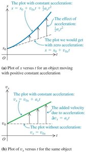
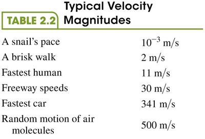
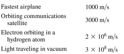
Summary Table: Typical Velocity Magnitudes

Situation	Velocity (m/s)
A snail's pace	$10^{-3}$
A brisk walk	2
Fastest human	11
Freeway speeds	30
Fastest car	341
Random motion of air molecules	500
Fastest airplane	1000
Orbiting communications satellite	3000
Electron orbiting in a hydrogen atom	$2 \times 10^6$
Light traveling in vacuum	$3 \times 10^8$

Summary Table: Signs of x-Velocity

If x-coordinate is:	x-velocity is:
Positive & increasing	Positive: Particle is moving in +x-direction
Positive & decreasing	Negative: Particle is moving in -x-direction
Negative & increasing	Positive: Particle is moving in +x-direction
Negative & decreasing	Negative: Particle is moving in -x-direction

Summary Table: Signs of x-Acceleration

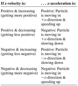
If x-velocity is:	x-acceleration is:
Positive & increasing	Positive: Particle is moving in +x-direction & speeding up
Positive & decreasing	Negative: Particle is moving in +x-direction & slowing down
Negative & increasing	Positive: Particle is moving in -x-direction & slowing down
Negative & decreasing	Negative: Particle is moving in -x-direction & speeding up

Summary Table: Kinematic Equations for Constant Acceleration

Equation	Includes Quantities
$v_x = v_{0x} + a_x t$	t, $v_x$, $a_x$
$x = x_0 + v_{0x} t + \frac{1}{2} a_x t^2$	t, x, $a_x$
$v_x^2 = v_{0x}^2 + 2 a_x (x - x_0)$	x, $v_x$, $a_x$
$x - x_0 = \frac{1}{2} (v_{0x} + v_x) t$	t, x, $v_x$

Example: Average and Instantaneous Velocities

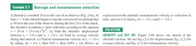
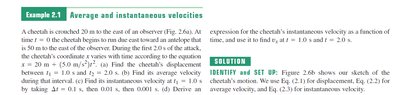
A cheetah is crouched 20 m to the east of an observer. During the first 2.0 s of the attack, its coordinate x varies with time according to $x = 20 \text{ m} + (5.0 \text{ m/s}) t - (0.50 \text{ m/s}^2) t^2$. Find the cheetah's displacement between t = 1.0 s and t = 2.0 s, its average velocity during that interval, and its instantaneous velocity at t = 1.0 s and t = 2.0 s.

Additional info: The notes cover all key aspects of Chapters 1 and 2, including vector analysis, kinematics, and motion with constant acceleration, with relevant examples and tables for exam preparation.