Concepts of Motion and Problem-Solving in Physics

Concepts of Motion

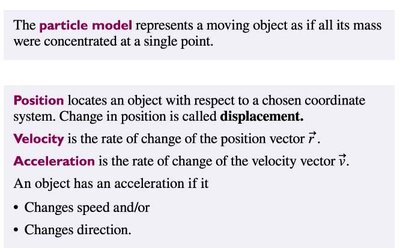
Particle Model and Motion Diagrams

The particle model simplifies a moving object by treating all its mass as if it were concentrated at a single point. This abstraction allows us to focus on the essential aspects of motion without unnecessary complexity.

• Position: Locates an object with respect to a chosen coordinate system. The change in position is called displacement.

• Velocity: The rate of change of the position vector $\vec{r}$.

• Acceleration: The rate of change of the velocity vector $\vec{v}$.

• An object has acceleration if it changes speed and/or direction.

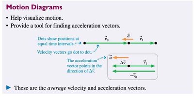
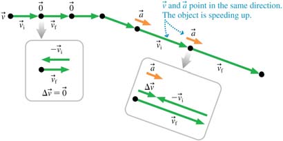
Motion Diagrams

Motion diagrams are visual tools that help us understand and analyze the motion of objects. They show the position of an object at equal time intervals, with velocity and acceleration vectors indicated.

• Dots represent positions at equal time intervals.

• Velocity vectors connect consecutive positions.

• Acceleration vectors show the change in velocity.

• These diagrams help identify whether an object is speeding up, slowing down, or moving at constant velocity.

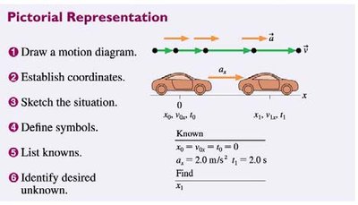
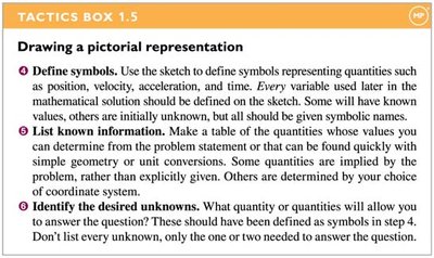
Pictorial Representation of Physics Problems

Elements of a Pictorial Representation

A pictorial representation of a physics problem organizes information visually and symbolically, making it easier to analyze and solve the problem. It typically includes:

• A sketch of the situation

• A coordinate system

• Symbols for physical quantities

• A table of known and unknown values

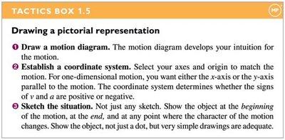
Steps for Drawing a Pictorial Representation

1. Draw a motion diagram: Develops intuition for the motion.

2. Establish a coordinate system: Select axes and origin to match the motion.

3. Sketch the situation: Show the object at the beginning, end, and any point where the motion changes.

4. Define symbols: Assign symbols for position, velocity, acceleration, and time.

5. List known information: Make a table of known quantities.

6. Identify desired unknowns: Specify the quantities to be found.

Analyzing Motion: Examples

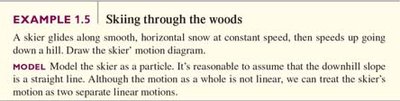
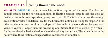
Example 1.5: Skiing Through the Woods

This example illustrates how to model and visualize the motion of a skier gliding on horizontal snow and then speeding up down a hill. The skier's motion is treated as two separate linear motions: constant speed on the flat and acceleration down the slope.

• Dots equally spaced for horizontal motion indicate constant speed.

• Dots farther apart on the slope indicate increasing speed (acceleration).

• Acceleration vectors are shown only where velocity changes.

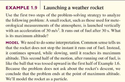
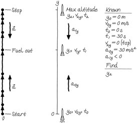
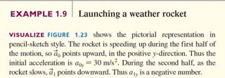
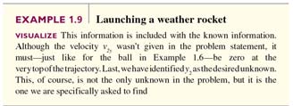
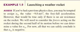
Example 1.9: Launching a Weather Rocket

This example demonstrates the use of pictorial representation and modeling to analyze the vertical motion of a rocket. The rocket accelerates upward while fuel burns, then continues upward while slowing down after fuel runs out, until it reaches maximum altitude.

• Knowns: Initial position, velocity, acceleration, and time intervals.

• Unknown: Maximum altitude reached by the rocket.

• Acceleration changes direction after fuel runs out (from positive to negative).

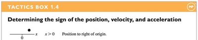
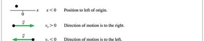
Position, Velocity, and Acceleration: Signs and Interpretation

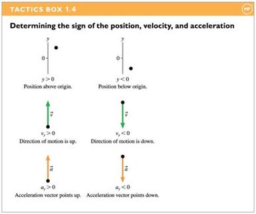
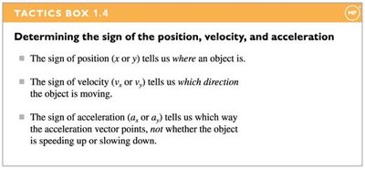
Determining the Sign of Position, Velocity, and Acceleration

The sign of each quantity provides information about the object's location and motion relative to the chosen coordinate system.

• Position (x or y): Indicates where the object is relative to the origin.

• Velocity (vx or vy): Indicates the direction of motion.

• Acceleration (ax or ay): Indicates the direction of the acceleration vector, not whether the object is speeding up or slowing down.

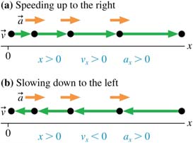
Speeding Up and Slowing Down

Whether an object is speeding up or slowing down depends on the relative directions of velocity and acceleration:

• If velocity and acceleration point in the same direction, the object speeds up.

• If velocity and acceleration point in opposite directions, the object slows down.

• Constant velocity occurs only when acceleration is zero.

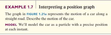
Position-versus-Time Graphs

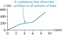
Interpreting Position Graphs

Position-versus-time graphs provide a visual representation of how an object's position changes over time. The slope of the graph at any point gives the object's velocity.

• A straight, sloped line indicates constant velocity.

• A curved line indicates changing velocity (acceleration).

• Horizontal segments indicate the object is at rest.

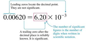
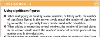
Significant Figures in Physics Calculations

Rules for Significant Figures

Significant figures reflect the precision of measured quantities and must be considered when reporting calculated results.

• When multiplying or dividing, the result should have as many significant figures as the least precisely known number.

• When adding or subtracting, the result should have as many decimal places as the number with the fewest decimal places.

• Leading zeros are not significant; trailing zeros after a decimal point are significant.

• Exact numbers do not affect the number of significant figures.

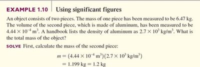
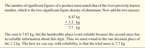
Example 1.10: Using Significant Figures

This example demonstrates how to apply significant figure rules in a calculation involving mass and density. The final answer is rounded to reflect the precision of the least certain measurement.

• Multiplication and addition are performed, with the result rounded to the correct number of significant figures.

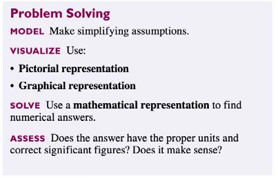
General Problem-Solving Strategy in Physics

Steps in Problem Solving

• Model: Make simplifying assumptions to focus on essential features.

• Visualize: Use pictorial and graphical representations to organize information.

• Solve: Develop a mathematical representation and solve for the unknowns.

• Assess: Check if the result is reasonable, has proper units, and correct significant figures.