Concepts of Motion: Foundations for Physics

Study Guide - Smart Notes

Tailored notes based on your materials, expanded with key definitions, examples, and context.

Concepts of Motion

Introduction to Motion

Motion is a fundamental concept in physics, describing the change in an object's position over time. Understanding motion is essential for analyzing a wide range of physical phenomena, from everyday activities to advanced scientific applications.

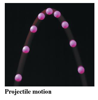
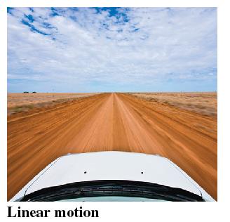
Translational Motion: The object moves through space, and its trajectory can be linear, parabolic, or circular.
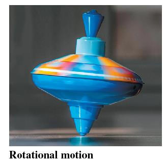
Rotational Motion: The object rotates about an axis but does not translate through space.
There are four basic types of motion commonly studied in physics: linear, projectile, circular, and rotational.

Cyclists in motion, illustrating translational motion Projectile motion: a ball following a parabolic path Linear motion: car moving straight on a road Circular motion: Ferris wheel at night Rotational motion: spinning top

Motion Diagrams

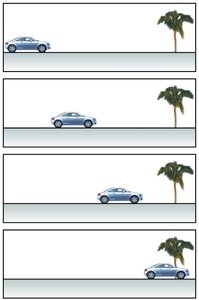
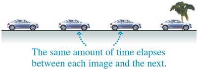
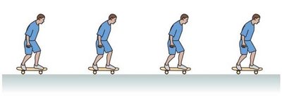
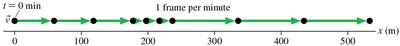
A motion diagram is a visual tool for analyzing motion by showing an object's position at several equally spaced instants of time. This helps in understanding how the position changes and whether the object is speeding up, slowing down, or moving at a constant speed.

Each frame in a motion diagram represents the object's position at a specific time.
Equally spaced images indicate constant speed, while increasing distances between images show acceleration.

Frames of a car moving past a tree, showing different positions at equal time intervals Composite image of car positions at equal time intervals Composite image of runners in a race, showing motion diagram Motion diagram: skateboarder at constant speed Motion diagram: runner speeding up

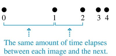
The Particle Model

To simplify the analysis of motion, objects are often modeled as particles, meaning all their mass is concentrated at a single point. This allows us to focus on the motion of the center of mass rather than the details of the object's shape or rotation.

The particle model is especially useful for objects moving in a straight line or following a simple trajectory.
Motion diagrams using the particle model show only the position of the particle at each time step.

Coordinate Systems and Position

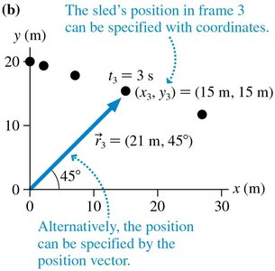
To describe motion precisely, a coordinate system is introduced. Each position is labeled with coordinates, such as (x, y), and the initial position is often labeled as point "0".

Positions are referenced relative to the chosen origin of the coordinate system.
Different observers may choose different coordinate systems, but the physical motion remains the same.

Motion diagram with coordinate system and position vector

Vectors and Scalars

Definitions and Examples

Physical quantities are classified as either scalars or vectors:

Scalar: A quantity described by a single number and unit (e.g., mass, time, temperature).
Vector: A quantity described by both magnitude and direction (e.g., velocity, acceleration, force).

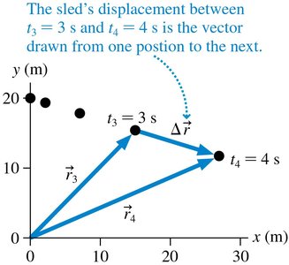
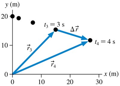
Position and Displacement Vectors

The position vector ($ \vec{r} $) locates an object relative to the origin. The displacement vector ($ \Delta \vec{r} $) points from the initial position to the final position, indicating both the distance and direction of motion.

Position vector at time $ t_3 $: $ \vec{r}_3 $
Displacement: $ \Delta \vec{r} = \vec{r}_4 - \vec{r}_3 $

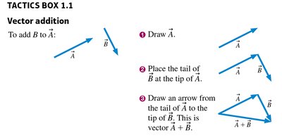
Position vector on a coordinate system Displacement vector between two positions

Vector Addition and Subtraction

Vectors can be added or subtracted graphically using the head-to-tail method. The resultant vector completes the triangle formed by the two vectors.

To add vectors $ \vec{A} $ and $ \vec{B} $, place the tail of $ \vec{B} $ at the tip of $ \vec{A} $.
To subtract, add the negative of the vector: $ \vec{A} - \vec{B} = \vec{A} + (-\vec{B}) $.

Tactics box: Vector addition

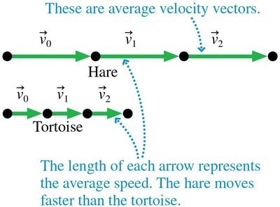
Displacement and Velocity in Motion Diagrams

In a motion diagram, displacement vectors connect each set of adjacent positions. The length of the displacement vector indicates the speed of the object.

Longer displacement vectors mean faster movement.
Velocity vectors are proportional to displacement vectors divided by the time interval.

Motion diagram with displacement vectors

Speed, Velocity, and Acceleration

Average Speed and Velocity

Average speed is the total distance traveled divided by the time taken. Average velocity is the displacement divided by the time interval, and it is a vector.

Average speed: $ \text{Average speed} = \frac{\text{distance traveled}}{\text{time taken}} = \frac{d}{\Delta t} $
Average velocity: $ \vec{v}_{\text{avg}} = \frac{\Delta \vec{r}}{\Delta t} $
Speed is the magnitude of the velocity vector.

Motion diagram with velocity vectors for tortoise and hare

Acceleration

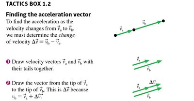
Acceleration is the rate of change of velocity. It is a vector and can be calculated as the change in velocity divided by the time interval.

Average acceleration: $ \vec{a}_{\text{avg}} = \frac{\vec{v}_2 - \vec{v}_1}{t_2 - t_1} = \frac{\Delta \vec{v}}{\Delta t} $
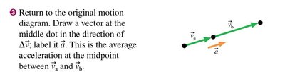
Acceleration vectors are drawn at the midpoint between two velocity vectors in a motion diagram.

Tactics box: Finding the acceleration vector Drawing the acceleration vector on a motion diagram

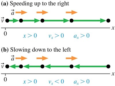
Speeding Up or Slowing Down

The direction of the acceleration vector relative to the velocity vector determines whether an object is speeding up or slowing down.

If acceleration and velocity point in the same direction, the object speeds up.
If they point in opposite directions, the object slows down.
If acceleration is zero, the object moves at constant speed.

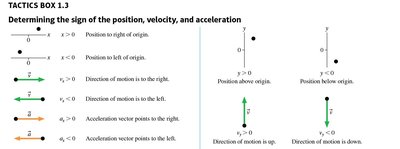
Speeding up and slowing down: acceleration and velocity directions

Signs of Position, Velocity, and Acceleration

The sign (positive or negative) of position, velocity, and acceleration depends on the chosen coordinate system. This helps in analyzing motion in different directions.

Tactics box: Determining the sign of position, velocity, and acceleration

Graphical Representation of Motion

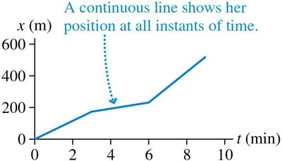
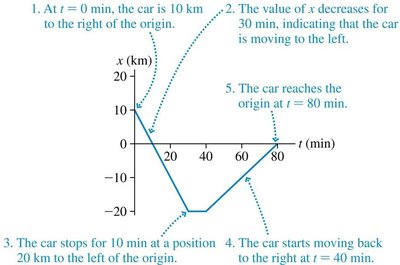
Position vs. Time Graphs

Position-time graphs provide a continuous representation of an object's motion. The slope of the graph at any point gives the object's velocity.

Steeper slopes indicate higher velocities.
Changes in slope indicate acceleration or deceleration.

Position vs. time graph: continuous line Position vs. time graph: motion diagram with velocity vectors Example: Interpreting a position vs. time graph for a car

Units and Measurement

SI Units

Physics relies on the International System of Units (SI), which standardizes measurements for scientific communication. The three fundamental SI units are the meter (m) for length, kilogram (kg) for mass, and second (s) for time.

Basic units: Length (meter), mass (kilogram), time (second), electric charge (coulomb).
Derived units: Formed from combinations of basic units (e.g., newton for force, joule for energy).
Prefixes are used for very large or small numbers (e.g., kilo-, milli-, micro-).

Atomic clock: standard of time International prototype kilogram

Unit Conversions

Unit conversions are essential for solving physics problems, especially when switching between SI and imperial units. Conversion factors are written as ratios and used to multiply the given value.

Imperial Unit	SI Equivalent
1 in	2.54 cm
1 mi	1.609 km
1 mph	0.447 m/s
1 m	39.37 in
1 km	0.621 mi
1 m/s	2.24 mph

Significant Figures

Precision and Reporting Results

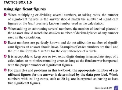
Significant figures reflect the precision of measurements and calculations. The number of significant figures in a result should not exceed that of the least precise measurement used in the calculation.

When multiplying or dividing, the result should have as many significant figures as the input with the fewest significant figures.
When adding or subtracting, the result should have as many decimal places as the input with the fewest decimal places.
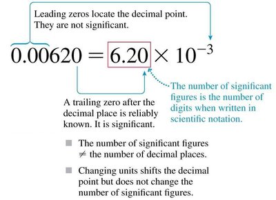
Scientific notation is used to clearly indicate the number of significant figures.

Tactics box: Using significant figures Example: Determining significant figures in scientific notation

Examples

Expressing 1200 kg to three significant figures: $1.20 \times 10^3$ kg
Expressing 0.0000340 s to three significant figures: $3.40 \times 10^{-5}$ s
When adding 6.47 kg and 1.2 kg, the result is rounded to 7.7 kg, reflecting the least precise value (1 decimal place).