Kinematics in One Dimension: Physics with Calculus Study Notes

Chapter 2: Kinematics in One Dimension

Introduction to Kinematics

Kinematics is the branch of mechanics that describes the motion of objects without considering the forces that cause the motion. In this chapter, we focus on motion along a straight line (one dimension), introducing key concepts such as position, velocity, and acceleration.

Uniform Motion

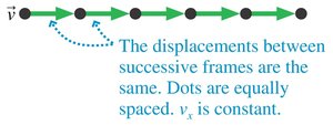
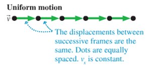
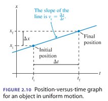
Uniform motion refers to straight-line motion in which equal displacements occur during any successive equal-time intervals. In this case, the velocity remains constant, and the position changes linearly with time.

• Definition: Motion with constant velocity (both magnitude and direction).

• Key Properties: Displacements between successive time intervals are equal; the position-versus-time graph is a straight line.

• Equation: $x_f = x_i + v_x \Delta t$

• Example: A car moving at a steady speed of 20 m/s along a straight road.

Position, Displacement, and Velocity

The position of an object is its location along a straight line, usually measured from a chosen origin. Displacement is the change in position, and velocity describes how quickly and in what direction the position changes.

• Displacement: $\Delta x = x_f - x_i$

• Average Velocity: $v_{avg} = \frac{\Delta x}{\Delta t}$

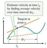
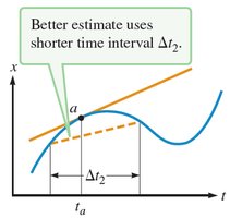
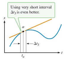
• Instantaneous Velocity: The velocity at a specific instant, found as the slope of the tangent to the position-versus-time graph at that point.

Velocity and Position Graphs

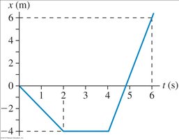
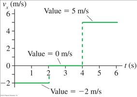
Graphs are essential tools in kinematics. The slope of a position-versus-time graph gives the velocity, while the area under a velocity-versus-time graph gives the displacement.

• Position-Time Graph: Slope = velocity.

• Velocity-Time Graph: Area under the curve = displacement.

• Turning Point: Where velocity is zero (object changes direction).

Instantaneous Velocity

Instantaneous velocity is the velocity of an object at a particular instant. It is found by taking the derivative of position with respect to time, or graphically, as the slope of the tangent to the position-time curve at a point.

• Mathematical Definition: $v_x = \lim_{\Delta t \to 0} \frac{\Delta x}{\Delta t}$

• Graphical Interpretation: Slope of the tangent line at a point on the x vs. t graph.

Motion with Constant Acceleration

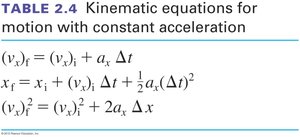
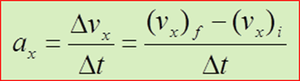
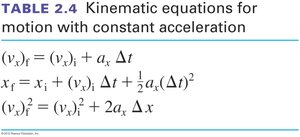
When an object's velocity changes at a constant rate, it is said to have constant acceleration. The kinematic equations describe the relationships between position, velocity, acceleration, and time for such motion.

• Acceleration: $a_x = \frac{\Delta v_x}{\Delta t}$

• Kinematic Equations:

Equation	Description
$v_{x,f} = v_{x,i} + a_x \Delta t$	Final velocity after time $\Delta t$
$x_f = x_i + v_{x,i} \Delta t + \frac{1}{2} a_x (\Delta t)^2$	Final position after time $\Delta t$
$v_{x,f}^2 = v_{x,i}^2 + 2 a_x \Delta x$	Velocity-position relationship (no time)

Graphical Analysis of Motion

Understanding the graphical relationships between position, velocity, and acceleration is crucial for analyzing motion:

• Slope of x-t graph: Velocity

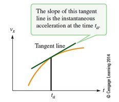
• Slope of v-t graph: Acceleration

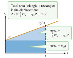
• Area under v-t graph: Displacement

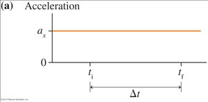
• Area under a-t graph: Change in velocity

Free Fall

Free fall is the motion of an object under the influence of gravity alone, with a constant acceleration directed downward. The acceleration due to gravity is denoted by $g$ and has a value of $9.80\ \mathrm{m/s^2}$ near Earth's surface.

• Key Point: All objects in free fall (neglecting air resistance) experience the same acceleration regardless of mass.

• Equations: Use the kinematic equations with $a = -g$ (downward direction).

Motion on an Inclined Plane

When an object moves along a frictionless inclined plane, the acceleration along the incline is a component of gravity: $a_x = \pm g \sin \theta$, where the sign depends on the direction of motion.

• Down the incline: $a_x = +g \sin \theta$

• Up the incline: $a_x = -g \sin \theta$

Problem-Solving Strategy in Kinematics

To solve kinematics problems, follow these steps:

1. Interpret the problem and identify what is being asked.

2. Draw a motion diagram or sketch the situation.

3. Establish a coordinate system and label known and unknown quantities.

4. List the relevant equations.

5. Solve algebraically before substituting numbers.

6. Check if the answer is reasonable.

Summary Table: Kinematic Quantities and Their Graphical Relationships

Quantity	Graphical Representation	Physical Meaning
Position (x)	y-axis on x-t graph	Location of object
Velocity (v)	Slope of x-t graph	Rate of change of position
Acceleration (a)	Slope of v-t graph	Rate of change of velocity
Displacement (Δx)	Area under v-t graph	Change in position

Key Equations (LaTeX Format)

• $v_{x,avg} = \frac{\Delta x}{\Delta t}$

• $v_x = \frac{dx}{dt}$

• $a_x = \frac{dv_x}{dt}$

• $x_f = x_i + v_{x,i} \Delta t + \frac{1}{2} a_x (\Delta t)^2$

• $v_{x,f} = v_{x,i} + a_x \Delta t$

• $v_{x,f}^2 = v_{x,i}^2 + 2 a_x \Delta x$

Applications and Examples

• Example 1: Calculating the displacement of a drag racer using the area under a velocity-time graph.

• Example 2: Determining the time and distance required for an airplane to take off using kinematic equations.

• Example 3: Analyzing the motion of a ball on an inclined plane using $a_x = g \sin \theta$.

Additional info: These notes include expanded academic context and explanations to ensure completeness and clarity for college-level Physics with Calculus students.