Kinematics in One Dimension: Structured Study Notes

Kinematics in One Dimension

Introduction to Kinematics

Kinematics is the branch of physics that describes the motion of objects without considering the forces that cause the motion. In one-dimensional kinematics, we focus on motion along a straight line, analyzing position, velocity, and acceleration as functions of time.

Graphical Representation in Kinematics

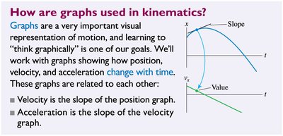
Graphs are essential tools in kinematics, providing visual representations of how position, velocity, and acceleration change with time. Understanding how to interpret and construct these graphs is fundamental for solving kinematics problems.

• Position vs. Time Graph: Shows how an object's position changes over time.

• Velocity vs. Time Graph: The slope of the position graph gives the velocity.

• Acceleration vs. Time Graph: The slope of the velocity graph gives the acceleration.

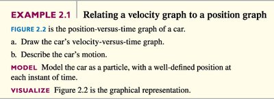
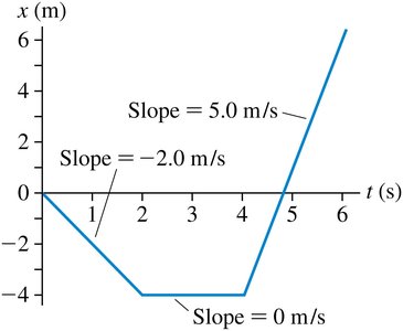
Relating Velocity and Position Graphs

To analyze motion, it is often necessary to relate velocity graphs to position graphs. The slope of the position-versus-time graph at any point gives the instantaneous velocity.

• Example: Given a position graph, draw the corresponding velocity graph and describe the motion.

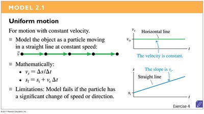
Uniform Motion Model

Uniform motion describes an object moving at a constant velocity along a straight line. This model is valid when the speed and direction do not change.

• Mathematical Description:

  • $v_s = \frac{\Delta s}{\Delta t}$

  • $s_f = s_i + v_s \Delta t$

• Limitations: The model fails if the particle's speed or direction changes significantly.

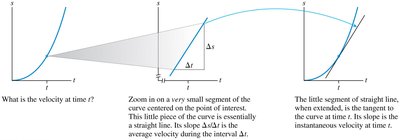
Instantaneous Velocity

Instantaneous velocity is the velocity of an object at a specific moment in time. It is found by taking the slope of the tangent to the position-versus-time curve at that point.

• Average Velocity: $v_{avg} = \frac{\Delta s}{\Delta t}$

• Instantaneous Velocity: $v = \lim_{\Delta t \to 0} \frac{\Delta s}{\Delta t}$

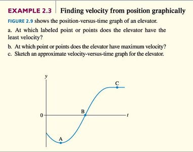
Finding Velocity from Position Graphically

By examining the position-versus-time graph, one can determine where the velocity is least or greatest and sketch the corresponding velocity graph.

• Maximum Velocity: Occurs where the slope is steepest.

• Zero Velocity: Occurs where the slope is zero (horizontal tangent).

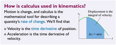
Calculus in Kinematics

Calculus provides a powerful framework for describing motion. The derivative of position with respect to time gives velocity, and the derivative of velocity gives acceleration. Conversely, integrating velocity over time yields displacement.

• Velocity: $v = \frac{d s}{d t}$

• Acceleration: $a = \frac{d v}{d t}$

• Displacement: $\Delta s = \int v \, dt$

Example: Using Calculus to Find Velocity

Given a position function $x(t)$, velocity can be found by differentiation. For example, if $x(t) = -t^2 + 3t$, then $v(t) = \frac{d x}{d t} = -2t + 3$.

• At $t = 2$ s: $x(2) = -4 + 6 = 2$ m, $v(2) = -4 + 3 = -1$ m/s

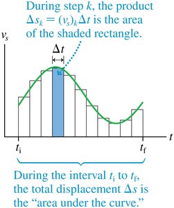
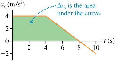
Displacement as Area Under the Curve

The total displacement during a time interval is the area under the velocity-versus-time curve. This can be calculated using integration or by summing areas of geometric shapes under the curve.

• For constant velocity: Area is a rectangle.

• For changing velocity: Area may be a combination of rectangles and triangles.

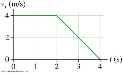
Example: Displacement During a Drag Race

To find how far a racer moves during a given time, calculate the area under the velocity graph for that interval.

• For a linear velocity function: The area under the curve is a triangle.

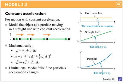
Constant Acceleration Model

When an object moves with constant acceleration, its motion can be described using kinematic equations. These equations relate position, velocity, acceleration, and time.

• $v_f = v_i + a \Delta t$

• $s_f = s_i + v_i \Delta t + \frac{1}{2} a (\Delta t)^2$

• $v_f^2 = v_i^2 + 2a \Delta s$

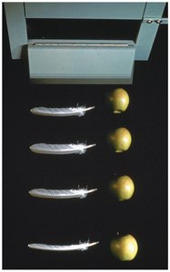
Free Fall

Free fall describes the motion of objects under the influence of gravity alone. All objects in free fall experience the same acceleration, $g = 9.8$ m/s2 on Earth, regardless of their mass (neglecting air resistance).

• Key Principle: In a vacuum, all objects fall at the same rate.

• Model: Free fall is modeled as motion with constant acceleration.

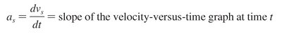
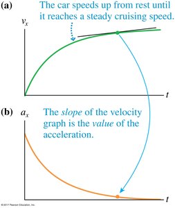
Instantaneous Acceleration

Instantaneous acceleration is the rate of change of velocity at a specific moment. It is found by taking the slope of the tangent to the velocity-versus-time curve.

• $a_s = \frac{d v_s}{d t}$

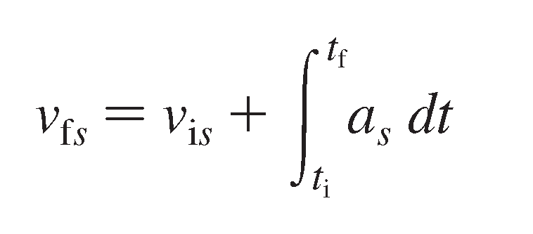
Advanced: Finding Velocity from Acceleration

If acceleration is known as a function of time, velocity can be found by integrating acceleration over the time interval.

• $v_{fS} = v_{iS} + \int_{t_i}^{t_f} a_S \, dt$

Summary Table: Kinematic Quantities and Their Relationships

Quantity	Graphical Representation	Mathematical Relationship
Position (s or x)	Position vs. Time	$v = \frac{d s}{d t}$
Velocity (v)	Velocity vs. Time	$a = \frac{d v}{d t}$
Acceleration (a)	Acceleration vs. Time	$\Delta v = \int a \, dt$
Displacement ($\Delta s$)	Area under velocity curve	$\Delta s = \int v \, dt$

Applications and Examples

• Example: Calculating impact velocity for a falling rock using kinematic equations.

• Example: Analyzing the motion of a rocket sled with changing acceleration.

• Example: Solving a two-car race problem using uniform motion and constant acceleration models.

Additional info: These notes expand on brief points from lecture slides and examples, providing academic context and formulas for a self-contained study guide.