Kinematics in Two Dimensions and Vectors: Study Notes

Chapter 3: Kinematics in Two Dimensions and Vectors

3-1 Vectors and Scalars

Kinematics in two dimensions requires understanding both vectors and scalars. Vectors are quantities that have both magnitude and direction, while scalars have only magnitude.

• Vector quantities: displacement, velocity, force, momentum

• Scalar quantities: mass, time, temperature

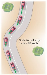
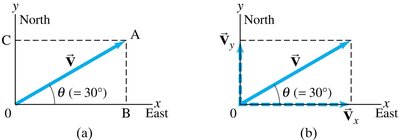
• Vectors are represented graphically by arrows; the length indicates magnitude and the arrow points in the direction.

3-2 Addition of Vectors—Graphical Methods

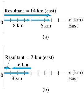
Vectors can be added graphically. In one dimension, simple addition and subtraction suffice, but in two dimensions, graphical methods are used.

• Collinear vectors: Add or subtract magnitudes, being careful with direction (sign).

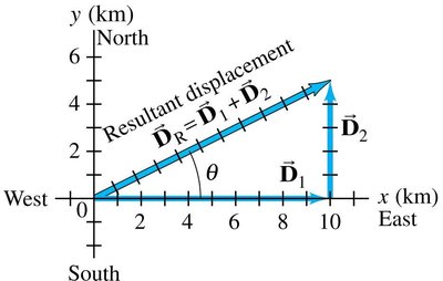
• Perpendicular vectors: Use the Pythagorean theorem to find the resultant.

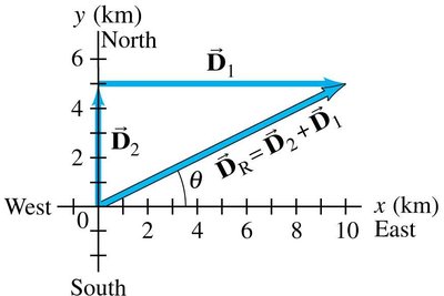
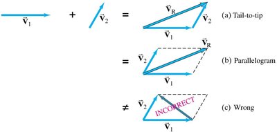
• Tail-to-tip method: Place the tail of the second vector at the tip of the first; the resultant is from the tail of the first to the tip of the last.

• Parallelogram method: Place vectors tail-to-tail and complete the parallelogram; the diagonal is the resultant.

• Order of addition does not affect the resultant vector.

3-3 Subtraction of Vectors, and Multiplication of a Vector by a Scalar

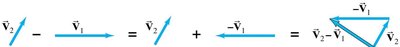
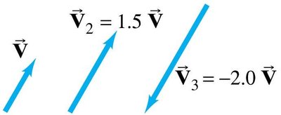
Vector subtraction is defined by adding the negative of a vector. Multiplying a vector by a scalar changes its magnitude but not its direction (unless the scalar is negative).

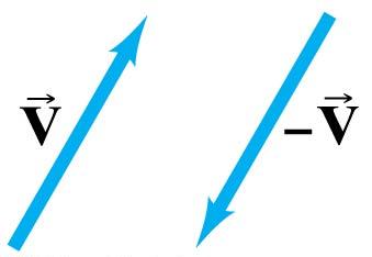
• Negative vector: Same magnitude, opposite direction.

• Subtraction: \( \vec{A} - \vec{B} = \vec{A} + (-\vec{B}) \)

• Scalar multiplication: \( c\vec{V} \) has magnitude \( |c|V \) and direction of \( \vec{V} \) if \( c > 0 \), opposite if \( c < 0 \).

3-4 Adding Vectors by Components

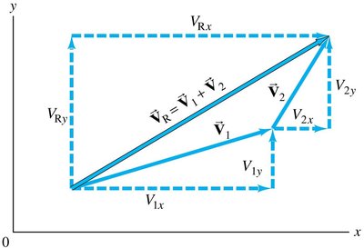
Any vector can be resolved into perpendicular components, usually along the x and y axes. This allows for algebraic addition of vectors by adding their respective components.

• Component form: \( \vec{V} = V_x \hat{i} + V_y \hat{j} \)

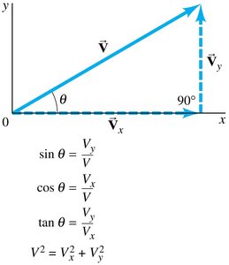
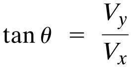
• Finding components: If \( \vec{V} \) makes an angle \( \theta \) with the x-axis:

$V_x = V \cos \theta$ $V_y = V \sin \theta$

• Magnitude and direction:

$V = \sqrt{V_x^2 + V_y^2}$ $\tan \theta = \frac{V_y}{V_x}$

• Adding vectors: Add x-components and y-components separately.

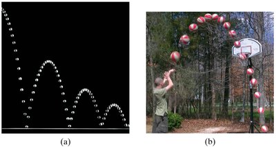
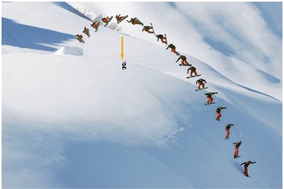
3-5 Projectile Motion

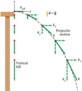
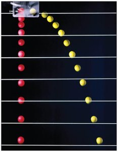
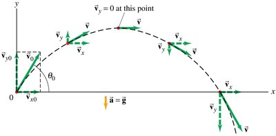
Projectile motion describes the motion of an object moving in two dimensions under the influence of gravity. The path is a parabola, and the horizontal and vertical motions are analyzed separately.

• Horizontal motion: Constant velocity (no horizontal acceleration).

• Vertical motion: Constant acceleration due to gravity (\( g \)).

• At the highest point, the vertical component of velocity is zero.

• Projectile motion can be solved by separating the x and y motions and using kinematic equations.

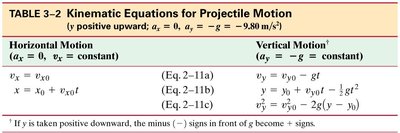
Kinematic Equations for Projectile Motion

	Horizontal Motion (a_x = 0, v_x = constant)	Vertical Motion (a_y = -g = constant)
Velocity	$v_x = v_{x0}$	$v_y = v_{y0} - gt$
Position	$x = x_0 + v_{x0} t$	$y = y_0 + v_{y0} t - \frac{1}{2}gt^2$
Velocity squared		$v_y^2 = v_{y0}^2 - 2g(y - y_0)$

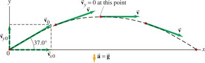
Example: Kicked Football

A football is kicked at an angle \( \theta_0 = 37.0^\circ \) with a velocity of 20.0 m/s. To find the maximum height, time of flight, and range:

• Resolve initial velocity into components:

$v_{x0} = v_0 \cos \theta_0$ $v_{y0} = v_0 \sin \theta_0$

• Use kinematic equations for vertical and horizontal motion.

Conceptual Questions

• Magnitude of a vector: Always positive; can only be zero if all components are zero.

• Projectile at highest point: Has the least speed (vertical velocity is zero).

• Horizontal range: For the same initial speed, a lower angle (but not too low) gives a greater range than a very steep angle.

• Cart firing a ball vertically: The ball lands back in the cart if there is no air resistance and the cart moves at constant velocity.

Summary Table: Key Properties of Vectors and Projectile Motion

Property	Vector	Scalar
Magnitude	Yes	Yes
Direction	Yes	No
Addition	Graphical or by components	Algebraic
Examples	Displacement, velocity, force	Mass, time, temperature

Additional info: The above notes expand on the graphical and analytical methods for vector addition, subtraction, and projectile motion, providing context and equations for solving typical physics problems in two dimensions.