Kinematics in Two Dimensions: Study Notes

Chapter 4: Kinematics in Two Dimensions

Introduction to Two-Dimensional Motion

Two-dimensional motion describes the movement of objects in a plane, involving both x and y directions. Unlike one-dimensional motion, objects can change both their speed and direction, requiring vector analysis to fully describe their trajectories.

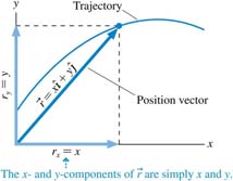
• Position Vector: The location of a particle in the xy-plane is given by the position vector \( \vec{r} \).

• Trajectory: The path followed by the particle is called its trajectory.

• Graphical Representation: Motion is often visualized as a graph of y versus x, showing the actual trajectory.

• Equation: \( \vec{r} = x \hat{i} + y \hat{j} \)

• Components: The x- and y-components of \( \vec{r} \) are simply x and y.

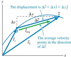
Displacement and Average Velocity

Displacement is the change in position of a particle, and average velocity is the rate of change of displacement over time. Both are vector quantities and are fundamental to understanding motion in two dimensions.

• Displacement: \( \Delta \vec{r} = \Delta x \hat{i} + \Delta y \hat{j} \)

• Average Velocity: Points in the direction of displacement and is given by \( \vec{v}_{avg} = \frac{\Delta \vec{r}}{\Delta t} \)

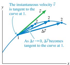
Instantaneous Velocity

The instantaneous velocity is the velocity of a particle at a specific moment and is tangent to the trajectory at that point. It is found by taking the limit as the time interval approaches zero.

• Definition: \( \vec{v} = \lim_{\Delta t \to 0} \frac{\Delta \vec{r}}{\Delta t} \)

• Component Form: \( \vec{v} = v_x \hat{i} + v_y \hat{j} \), where \( v_x = \frac{dx}{dt} \) and \( v_y = \frac{dy}{dt} \)

• Direction: The instantaneous velocity vector is always tangent to the trajectory.

Velocity Components and Speed

Velocity in two dimensions can be broken down into x and y components. The speed is the magnitude of the velocity vector, and the direction can be determined from the components.

• Velocity Components: \( v_x = v \cos \theta \), \( v_y = v \sin \theta \)

• Speed: \( v = \sqrt{v_x^2 + v_y^2} \)

• Direction: \( \theta = \tan^{-1} \left( \frac{v_y}{v_x} \right) \)

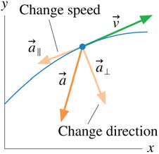
Acceleration in Two Dimensions

Acceleration is the rate of change of velocity. In two dimensions, acceleration can change the speed (magnitude of velocity) or the direction of motion, or both. The acceleration vector points in the direction of the change in velocity.

• Average Acceleration: \( \vec{a}_{avg} = \frac{\Delta \vec{v}}{\Delta t} \)

• Components: Acceleration can be decomposed into components parallel (tangential) and perpendicular (normal) to the trajectory.

• Graphical Representation: The parallel component changes speed, while the perpendicular component changes direction.

Projectile Motion

Projectile motion is a classic example of two-dimensional motion under the influence of gravity. The trajectory is parabolic, with uniform motion in the horizontal direction and constant acceleration in the vertical direction.

• Horizontal Motion: \( a_x = 0 \), velocity is constant.

• Vertical Motion: \( a_y = -g \), where g is the acceleration due to gravity.

• Trajectory: Parabolic path.

• Equation: \( y = y_0 + v_{y0} t - \frac{1}{2} g t^2 \)

Relative Motion and Reference Frames

Relative motion describes how the velocity of an object changes depending on the observer's reference frame. The velocity of an object in one frame can be found by vector addition of velocities from different frames.

• Reference Frames: Coordinate systems that move relative to each other.

• Velocity Addition: \( \vec{v}_{CB} = \vec{v}_{CA} + \vec{v}_{AB} \)

• Application: Used in problems involving moving platforms, vehicles, or fluids.

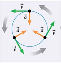
Circular Motion and Centripetal Acceleration

Circular motion involves movement along a circular path, characterized by angular displacement, angular velocity, and angular acceleration. Centripetal acceleration points toward the center of the circle and is responsible for changing the direction of velocity.

• Angular Velocity: \( \omega \), analogous to linear velocity.

• Angular Acceleration: \( \alpha \), analogous to linear acceleration.

• Centripetal Acceleration: \( a_c = \frac{v^2}{r} \), always directed toward the center.

• Tangential Acceleration: Present if speed changes.

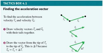
Finding the Acceleration Vector

To determine the acceleration vector between two velocity vectors, use vector subtraction. This process is essential for analyzing changes in velocity in two-dimensional motion.

• Step 1: Draw velocity vectors \( \vec{v}_a \) and \( \vec{v}_b \) with their tails together.

• Step 2: Draw the vector from the tip of \( \vec{v}_a \) to the tip of \( \vec{v}_b \). This is \( \Delta \vec{v} \).

• Equation: \( \vec{v}_b = \vec{v}_a + \Delta \vec{v} \)

Applications of Two-Dimensional Motion

Two-dimensional motion is ubiquitous in physics and everyday life. Examples include the motion of balls, cars turning corners, planetary orbits, and electrons spiraling in magnetic fields.

• Examples: Sports, vehicle navigation, astronomy, electromagnetism.

• Importance: Understanding two-dimensional motion is essential for analyzing real-world phenomena.