Kinematics: Motion in One Dimension – Study Notes

Chapter 2: Kinematics – Motion in One Dimension

2.1 What Is Motion?

Kinematics is the branch of physics that describes the motion of objects without considering the causes of motion. Motion is always described relative to a chosen observer and reference frame.

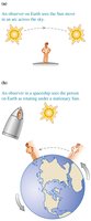
• Motion is Relative: The description of an object's motion depends on the observer's frame of reference. For example, the Sun appears to move across the sky for an observer on Earth, but an observer in a spaceship may see the Earth rotating under a stationary Sun.

• Reference Frame: A reference frame consists of an object of reference, a coordinate system for measuring distances, and a clock for measuring time. It is essential to specify the reference frame before describing motion.

• Modeling Motion: To simplify analysis, objects are often modeled as point-like and their motion as linear (along a straight line).

2.2 A Conceptual Description of Motion

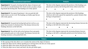
Understanding motion begins with qualitative observations and visual representations, such as motion diagrams and dot patterns.

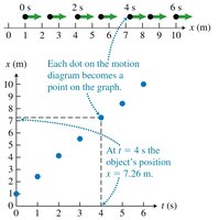
• Motion Diagrams: Dots represent the position of an object at equal time intervals. The spacing of the dots indicates the object's speed and changes in motion.

• Patterns: Evenly spaced dots indicate constant velocity; increasing or decreasing spacing indicates acceleration or deceleration.

2.3 Operations with Vectors

Vectors are quantities with both magnitude and direction, essential for describing displacement, velocity, and acceleration in physics.

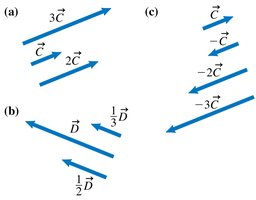
• Vector Representation: The length of the arrow shows magnitude; the arrow points in the direction of the vector.

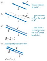
• Adding Vectors: Use the tail-to-head method: place the tail of one vector at the head of another to find the resultant vector.

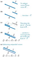
• Subtracting Vectors: To subtract, add the negative of the vector (reverse its direction).

• Multiplying by a Scalar: Multiplying a vector by a positive scalar changes its magnitude but not its direction; a negative scalar reverses the direction.

2.4 Quantities for Describing Motion

To analyze motion quantitatively, several key quantities are defined:

• Time (t): A clock reading; measured in seconds (s).

• Time Interval (\( \Delta t \)): The difference between two clock readings: $\Delta t = t_2 - t_1$

• Position (x): The location of an object relative to the origin of the coordinate system.

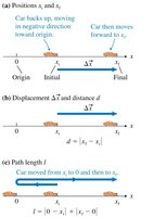
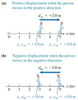
• Displacement (\( \Delta x \)): The change in position: $\Delta x = x_f - x_i$ (vector quantity).

• Distance: The magnitude of displacement (always positive).

• Path Length: The actual length of the path traveled, which may differ from displacement if the path is not straight.

2.5 Representing an Object’s Position with Data Tables and Graphs

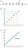
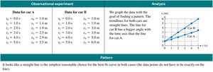
Motion can be represented using data tables and graphs, which help identify patterns and relationships between position and time.

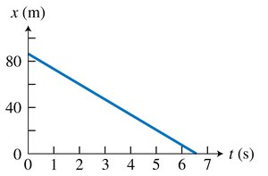
• Position-vs-Time Graphs: Time is plotted on the horizontal axis (independent variable), and position on the vertical axis (dependent variable).

• Trendline: A best-fit line or curve that summarizes the overall pattern of the data.

• Correspondence: Each dot in a motion diagram corresponds to a point on the position axis of the graph.

2.6 Constant Velocity Linear Motion

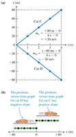
When an object moves with constant velocity, its position changes linearly with time.

• Equation of Motion: $x = x_0 + v_x t$ where $x_0$ is the initial position, $v_x$ is the constant velocity, and $t$ is time.

• Graphical Representation: The position-vs-time graph is a straight line; the slope equals the velocity.

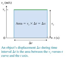
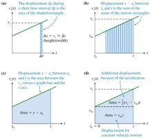
• Displacement from Velocity Graph: The area under a velocity-vs-time graph gives the displacement: $\Delta x = v_x \Delta t$

2.7 Motion at Changing Velocity (Acceleration)

When velocity changes, the object is said to accelerate. Acceleration is the rate of change of velocity with respect to time.

• Average Velocity: $\bar{v} = \frac{\Delta x}{\Delta t}$

• Instantaneous Velocity: The velocity at a specific instant; for constant velocity, average and instantaneous velocities are equal.

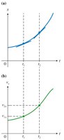
• Acceleration (a): $a = \frac{\Delta v}{\Delta t}$ (vector quantity)

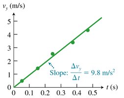
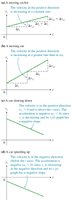
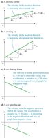
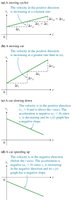
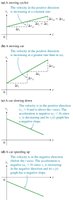
• Constant Acceleration: The velocity-vs-time graph is a straight line; the slope gives the acceleration.

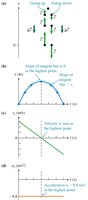
2.8 Displacement of an Object Moving at Constant Acceleration

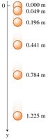
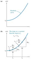
For motion with constant acceleration, the position as a function of time is given by a quadratic equation.

• Equation of Motion: $x = x_0 + v_{0x} t + \frac{1}{2} a_x t^2$

• Velocity Equation: $v_x = v_{0x} + a_x t$

• Graphical Representation: The position-vs-time graph is a parabola; the slope at any point gives the instantaneous velocity.

• Displacement without Time: $v_x^2 = v_{0x}^2 + 2 a_x (x - x_0)$

2.9 Skills for Analyzing Situations Involving Motion

Effective problem-solving in kinematics involves representing the situation in multiple ways and following a systematic approach.

• Step 1: Sketch and Translate – Draw the scenario, choose the object of interest, and set up a coordinate system.

• Step 2: Simplify and Diagram – Decide on the model (point-like object, constant velocity/acceleration), and draw diagrams or graphs as needed.

• Step 3: Represent Mathematically – Use equations and consider the sign of each quantity to solve the problem.

Summary of Key Concepts

• Position (x): Scalar, location relative to origin.

• Displacement (\( \Delta x \)): Vector, change in position.

• Distance (d): Scalar, magnitude of displacement.

• Path Length (l): Actual length traveled.

• Velocity (v): Vector, rate of change of position.

• Speed: Scalar, magnitude of velocity.

• Acceleration (a): Vector, rate of change of velocity.

Quantity	Definition	Equation	SI Unit
Displacement	Change in position	$\Delta x = x_f - x_i$	m
Average Velocity	Displacement per unit time	$\bar{v} = \frac{\Delta x}{\Delta t}$	m/s
Average Acceleration	Change in velocity per unit time	$a = \frac{\Delta v}{\Delta t}$	m/s^2
Position (constant velocity)	Linear function of time	$x = x_0 + v_x t$	m
Position (constant acceleration)	Quadratic function of time	$x = x_0 + v_{0x} t + \frac{1}{2} a_x t^2$	m
Velocity (constant acceleration)	Linear function of time	$v_x = v_{0x} + a_x t$	m/s
Velocity squared	Relates velocity and displacement	$v_x^2 = v_{0x}^2 + 2 a_x (x - x_0)$	m^2/s^2

Example: A car starts from rest ($v_{0x} = 0$) and accelerates at $2\ \mathrm{m/s^2}$ for $5\ \mathrm{s}$. Find its displacement.

• Use $x = x_0 + v_{0x} t + \frac{1}{2} a_x t^2$

• Assume $x_0 = 0$:

• $x = 0 + 0 \times 5 + \frac{1}{2} \times 2 \times 5^2 = 25\ \mathrm{m}$

Additional info: These notes cover the foundational concepts of one-dimensional kinematics, including the use of vectors, graphical analysis, and equations of motion for both constant velocity and constant acceleration. Mastery of these concepts is essential for further study in Newtonian mechanics and other areas of physics.