Kinematics: Motion with Constant Acceleration and Free-Fall

Motion Along a Straight Line

Introduction to Kinematics

Kinematics is the branch of physics that describes the motion of objects without considering the causes of motion. It focuses on quantities such as displacement, velocity, and acceleration, and their relationships through time.

• Displacement (x): The change in position of an object.

• Velocity (v): The rate of change of displacement with respect to time.

• Acceleration (a): The rate of change of velocity with respect to time.

Equations of Motion with Constant Acceleration

Kinematic Equations

When an object moves with constant acceleration, its motion can be described by a set of kinematic equations. These equations relate displacement, initial velocity, final velocity, acceleration, and time.

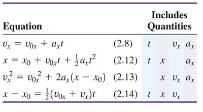
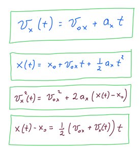
• First Equation (Velocity-Time): $v_x = v_{0x} + a_x t$

• Second Equation (Position-Time): $x = x_0 + v_{0x} t + \frac{1}{2} a_x t^2$

• Third Equation (Velocity-Displacement): $v_x^2 = v_{0x}^2 + 2 a_x (x - x_0)$

• Fourth Equation (Displacement-Average Velocity): $x - x_0 = \frac{1}{2} (v_{0x} + v_x) t$

Key Point: These equations are only valid for motion with constant acceleration.

Derivation of Kinematic Equations

The kinematic equations can be derived using algebraic manipulation and calculus. For example, integrating acceleration with respect to time yields velocity, and integrating velocity yields position.

• Velocity from Acceleration: $v_x = \int a_x dt = a_x t + v_{0x}$

• Position from Velocity: $x = \int v_x dt = x_0 + v_{0x} t + \frac{1}{2} a_x t^2$

Velocity and Position by Integration

Using Calculus in Kinematics

Integration is a powerful tool in kinematics, allowing us to determine velocity and position functions when acceleration is known. For constant acceleration, the integration process leads directly to the standard kinematic equations.

• General Approach: Integrate acceleration to get velocity, then integrate velocity to get position.

• Example: If $a_x$ is constant, then $v_x = v_{0x} + a_x t$ and $x = x_0 + v_{0x} t + \frac{1}{2} a_x t^2$.

Motion with Constant Acceleration: Example Problem

Antelope Problem

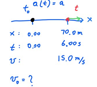
Example 2.19: An antelope moving with constant acceleration covers the distance between two points 70.0 m apart in 6.00 s. Its speed as it passes the second point is 15.0 m/s. What are (a) its speed at the first point and (b) its acceleration?

• Given: $x_0 = 0$, $x = 70.0$ m, $t = 6.00$ s, $v = 15.0$ m/s

• Find: $v_0$ and $a$

• Solution Strategy: Use the kinematic equations to solve for the unknowns. First, use the velocity-time equation to relate $v_0$, $a$, and $t$. Then, use the position-time equation to relate $x$, $x_0$, $v_0$, $a$, and $t$.

Step-by-step:

1. Write the equations:

   • $v = v_0 + a t$

   • $x = x_0 + v_0 t + \frac{1}{2} a t^2$

2. Substitute known values and solve the system of equations for $v_0$ and $a$.

Significant Figures: Always report answers with the correct number of significant figures based on the data provided.

Freely Falling Objects

Acceleration Due to Gravity

Objects in free-fall near the Earth's surface experience a constant acceleration directed downward, called the acceleration due to gravity, denoted as $g$.

• Value: $g = 9.8$ m/s2 (downward)

• Sign Convention: If upward is positive, then $a_y = -g = -9.8$ m/s2

• Key Point: All objects in free-fall (neglecting air resistance) experience the same acceleration regardless of their mass.

Equations for Free-Fall Motion

The kinematic equations apply to free-fall motion, with $a$ replaced by $-g$.

• $v_y = v_{0y} - g t$

• $y = y_0 + v_{0y} t - \frac{1}{2} g t^2$

• $v_y^2 = v_{0y}^2 - 2g(y - y_0)$

Example: Rock Thrown Upward

You throw a rock straight up from the edge of a cliff. It leaves your hand at time $t = 0$ moving at 16.0 m/s. Air resistance can be neglected. Find the time at which the rock is 4.00 m above where it left your hand.

• Given: $v_{0y} = 16.0$ m/s, $y - y_0 = 4.00$ m, $g = 9.8$ m/s2

• Find: $t$

• Solution: Use $y = y_0 + v_{0y} t - \frac{1}{2} g t^2$ and solve for $t$.

Summary Table: Kinematic Equations for Constant Acceleration

Equation	Includes Quantities
$v_x = v_{0x} + a_x t$	$t, v_x, a_x$
$x = x_0 + v_{0x} t + \frac{1}{2} a_x t^2$	$t, x, v_{0x}, a_x$
$v_x^2 = v_{0x}^2 + 2 a_x (x - x_0)$	$x, v_x, a_x$
$x - x_0 = \frac{1}{2} (v_{0x} + v_x) t$	$t, x, v_x$

Key Problem-Solving Strategies

• Identify known and unknown quantities.

• Choose the appropriate kinematic equation based on the variables involved.

• Solve algebraically for the unknown before substituting numerical values.

• Check units and significant figures in your final answer.

Example Application: These strategies are essential for solving real-world physics problems involving motion, such as calculating the time for a projectile to reach a certain height or the initial speed of a moving object.

Additional info: The notes also reference the use of simulations (e.g., PhET Moving Man) to visualize motion, which can help reinforce understanding of kinematic concepts.