 Back
BackLinear Motion: Speed, Velocity, and Position in One Dimension
Study Guide - Smart Notes
 Tailored notes based on your materials, expanded with key definitions, examples, and context.
Algebraic Manipulation and Solving for Values
Solving for Values in Physics Equations
Physics often requires solving for unknown variables using algebraic manipulation. This skill is essential for understanding relationships between physical quantities and for solving problems efficiently.
Key Point 1: Rearranging equations allows you to isolate the desired variable. For example, to solve for velocity () in the equation , substitute known values for displacement () and time ().
Key Point 2: Use algebraic manipulation to solve for mass () in kinetic energy equations: .
Example: If and , then .
Unit Prefixes and Scientific Notation
Understanding Unit Prefixes
Unit prefixes are used to express quantities in powers of ten, making it easier to handle very large or small numbers in physics.
Key Point 1: Common prefixes include kilo (), milli (), micro (), and so on.
Key Point 2: Scientific notation expresses numbers as a product of a coefficient and a power of ten, e.g., .
Example: .
Linear Motion – Speed and Velocity
Motion in One Dimension (1D)
Linear motion refers to movement along a straight line, described by position, displacement, speed, and velocity. Understanding 1D motion is foundational for analyzing more complex motion in physics.
Key Point 1: Motion is the change in position of an object over time.
Key Point 2: 1D motion occurs along a single axis, such as horizontal or vertical movement.
Example: A train moving along a straight track is an example of 1D motion.

Frames of Reference and Relative Motion
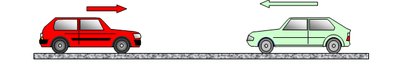
Motion is always measured relative to a chosen frame of reference. An inertial frame of reference is one in which Newton's laws hold true.
Key Point 1: The same motion can appear different depending on the observer's frame of reference.
Key Point 2: Establishing a frame of reference is crucial for accurate measurement and analysis.
Example: A car moving east at 100 km/h relative to the ground, but at 200 km/h relative to another car moving west at 100 km/h.

Distance vs. Displacement
Definitions and Differences
Distance and displacement are fundamental concepts in describing motion. Distance is a scalar quantity, while displacement is a vector.
Key Point 1: Distance is the total length traveled, regardless of direction.
Key Point 2: Displacement is the straight-line change in position from the initial to the final point, including direction.
Example: Walking 10 meters east and then 10 meters west results in a distance of 20 meters but a displacement of 0 meters.
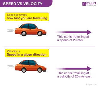
Speed vs. Velocity
Comparing Scalar and Vector Quantities
Speed and velocity both describe how fast an object moves, but velocity also includes direction.
Key Point 1: Speed is the rate of change of distance, a scalar quantity.
Key Point 2: Velocity is the rate of change of displacement, a vector quantity.
Example: A car moving at 20 m/s east has a speed of 20 m/s and a velocity of 20 m/s east.
Instantaneous vs. Average Speed and Velocity
Understanding Time Scales
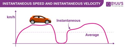
Instantaneous speed or velocity refers to the value at a specific moment, while average speed or velocity is calculated over a time interval.
Key Point 1: Instantaneous speed is measured at a particular instant.
Key Point 2: Average speed is total distance divided by total time; average velocity is total displacement divided by total time.
Example: A cheetah sprints 100 meters in 4 seconds: average speed = .

Mathematical Representation of Motion
Equations for Speed and Velocity
Motion can be described mathematically using equations that relate position, time, speed, and velocity.
Key Point 1: Average speed: , where is distance and is time.
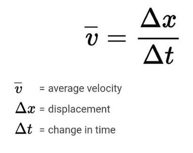
Key Point 2: Average velocity: , where is displacement and is change in time.
Example: If displacement is 1176 m and time is 1200 s, average velocity = .
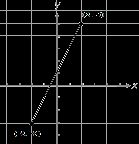
Position vs. Time Graphs
Interpreting Position-Time Plots
Position vs. time graphs visually represent how an object's position changes over time. The slope of the graph indicates velocity.
Key Point 1: A straight line indicates constant velocity; the slope equals velocity.
Key Point 2: A horizontal line indicates zero velocity (object at rest).
Example: If position changes from 0 m to 2 m in 2.5 s, average velocity = .
Equations of Motion
Linear Equations for Position
For constant velocity, position as a function of time can be written as .
Key Point 1: The equation describes linear motion.
Key Point 2: The slope of a position-time graph represents velocity.
Example: A ball starting at 4 m with velocity 2 m/s: .

Example Problems and Applications
Solving Linear Motion Problems
Applying the concepts of speed, velocity, and displacement to real-world problems helps reinforce understanding.
Key Point 1: Identify known values, required unknowns, and relevant equations.
Key Point 2: Convert units as necessary and manipulate equations to solve for the unknown.
Example: Two runners, one at 1 m/s and another at 2 m/s, determine when the second runner is 6 m ahead: .
Unit Conversions
Converting Between Units
Unit conversions are essential for ensuring consistency in calculations. Use unit prefixes and conversion factors to switch between units.
Key Point 1: To convert grams to kilograms, divide by 1000: .
Key Point 2: To convert meters per second to centimeters per hour: .
Summary Table: Unit Prefixes
Memorize Common Prefixes
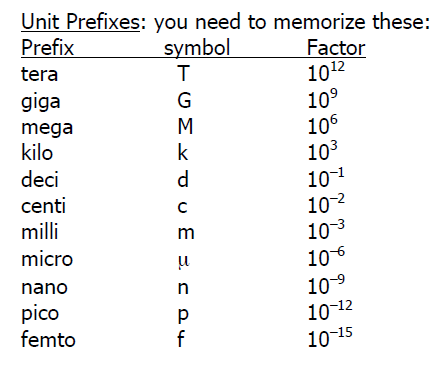
The following table summarizes the most common unit prefixes used in physics:
Prefix | Symbol | Factor |
|---|---|---|
tera | T | |
giga | G | |
mega | M | |
kilo | k | |
deci | d | |
centi | c | |
milli | m | |
micro | μ | |
nano | n | |
pico | p | |
femto | f |
Additional info: These notes cover foundational concepts from Chapter 3 (Linear Motion) and related algebraic skills, unit conversions, and graphical analysis, which are essential for college-level physics.
