Models, Measurements, and Vectors: Foundations for Physics with Calculus

Models, Measurements & Vectors

Introduction to Physical Quantities and Vectors

Physics uses models and measurements to describe the natural world quantitatively. Vectors are essential mathematical tools for representing quantities that have both magnitude and direction, such as displacement, velocity, and force.

Scalar and Vector Quantities

• Scalar Quantity: A physical quantity described by magnitude only (e.g., mass, temperature, distance).

• Vector Quantity: A physical quantity described by both magnitude and direction (e.g., displacement, velocity, force).

Displacement vs. Distance

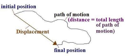
Distance is the total length of the path traveled, while displacement is the straight-line vector from the initial to the final position.

• Distance: Scalar, always positive, path-dependent.

• Displacement: Vector, can be positive or negative, depends only on initial and final positions.

• Formula: $\Delta \vec{r} = \vec{r}_f - \vec{r}_i$

Vector Representation and Direction

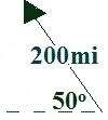
Vectors are represented by arrows. The length indicates magnitude, and the arrowhead shows direction. Directions are often given using angles measured from a reference axis (e.g., the positive x-axis or East).

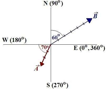
• Standard Position: Vectors are often drawn with their tail at the origin.

• Angle Measurement: Angles are measured counterclockwise from the positive x-axis (East).

Quadrants in the Coordinate System

The Cartesian plane is divided into four quadrants, which help in determining the signs of vector components.

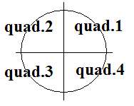
• Quadrant I: (+x, +y)

• Quadrant II: (−x, +y)

• Quadrant III: (−x, −y)

• Quadrant IV: (+x, −y)

Resolving Vectors into Components

Any vector can be broken down into perpendicular components, usually along the x and y axes. This process is called vector resolution.

Resolving Along the x-axis

1. Draw the x-axis from the vector's tail.

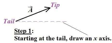
2. From the tip, draw a perpendicular to the x-axis (projection point).

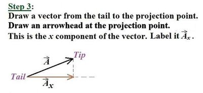
3. Draw the x-component from the tail to the projection point.

Resolving Along the y-axis

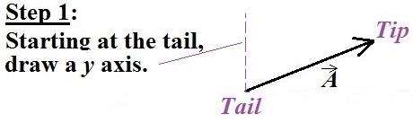
1. Draw the y-axis from the vector's tail.

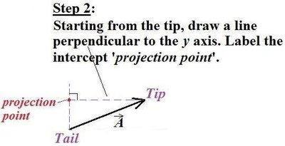
2. From the tip, draw a perpendicular to the y-axis (projection point).

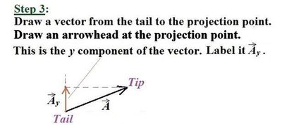
3. Draw the y-component from the tail to the projection point.

• Component Formulas:

  • $A_x = A \cos \theta$

  • $A_y = A \sin \theta$

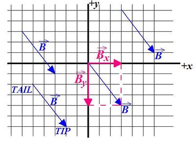
Graphical Representation of Vector Components

Vectors and their components can be visualized on a grid, which helps in understanding their addition and resolution.

Examples of Vector Resolution

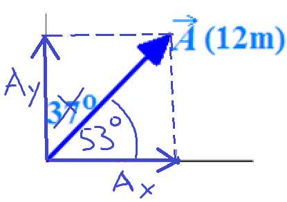
• Example 1: Given $\vec{A}$ with magnitude 12 m at 37° above the x-axis:

  • $A_x = 12 \cos 37^\circ$

  • $A_y = 12 \sin 37^\circ$

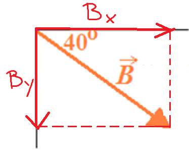
• Example 2: Given $\vec{B}$ with magnitude 15 m at 40° below the x-axis:

  • $B_x = 15 \cos 40^\circ$

  • $B_y = -15 \sin 40^\circ$

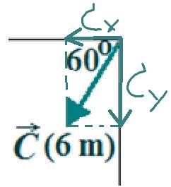
• Example 3: Given $\vec{C}$ with magnitude 6 m at 60° below the x-axis:

  • $C_x = 6 \cos 60^\circ$

  • $C_y = -6 \sin 60^\circ$

Vector Addition and Subtraction

Vectors can be added graphically (tip-to-tail method) or analytically (by adding components). Subtraction is performed by adding the negative of a vector.

• Resultant Vector: $\vec{R} = \vec{A} + \vec{B}$

• Component Addition:

  • $R_x = A_x + B_x$

  • $R_y = A_y + B_y$

• Magnitude: $R = \sqrt{R_x^2 + R_y^2}$

• Direction: $\theta = \tan^{-1}\left(\frac{R_y}{R_x}\right)$

Summary Table: Scalar vs. Vector Quantities

Quantity	Scalar	Vector
Distance/Displacement	Distance	Displacement
Speed/Velocity	Speed	Velocity
Mass/Weight	Mass	Weight
Energy/Force	Energy	Force

Key Takeaways

• Vectors are fundamental in describing physical phenomena involving direction and magnitude.

• Resolving vectors into components simplifies calculations in physics problems.

• Understanding the difference between scalar and vector quantities is crucial for accurate physical modeling.