Motion Along a Straight Line: Displacement, Velocity, and Acceleration

Motion Along a Straight Line

Displacement, Time, and Average Velocity

Motion along a straight line is a fundamental topic in kinematics, focusing on how objects move in one dimension. The displacement, time interval, and average velocity are key quantities used to describe such motion.

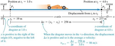
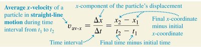
• Displacement (Δx): The change in position of a particle along the x-axis, defined as Δx = x2 - x1.

• Time Interval (Δt): The difference between the final and initial times, Δt = t2 - t1.

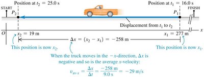
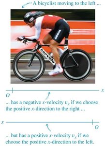
• Average Velocity (vav-x): The rate of change of displacement over time, given by: $v_{\text{av-x}} = \frac{\Delta x}{\Delta t} = \frac{x_2 - x_1}{t_2 - t_1}$ The sign of velocity indicates direction: positive for motion in the +x direction, negative for motion in the -x direction.

• Example: A dragster moves from x1 = 19 m at t1 = 1.0 s to x2 = 277 m at t2 = 4.0 s. The displacement is Δx = 258 m and the average velocity is 86 m/s.

Position-Time Graphs and Velocity

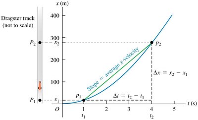
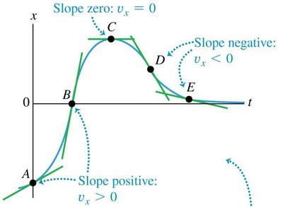
Position-time (x-t) graphs are used to visualize motion. The slope of the graph represents the average velocity over a time interval.

• Slope Interpretation: The slope between two points (x1, t1) and (x2, t2) gives the average velocity.

• Direction: Positive slope indicates motion in the +x direction; negative slope indicates motion in the -x direction.

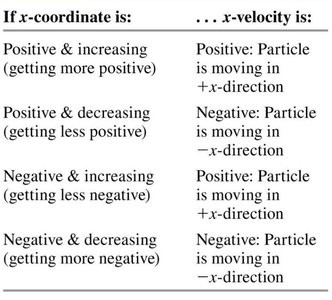
Rules for the Sign of x-Velocity

The sign of the x-velocity depends on the direction and change of the x-coordinate.

• Positive & Increasing: Moving in +x direction.

• Positive & Decreasing: Moving in -x direction.

• Negative & Increasing: Moving in +x direction.

• Negative & Decreasing: Moving in -x direction.

If x-coordinate is:	x-velocity is:
Positive & increasing	Positive: Particle is moving in +x-direction
Positive & decreasing	Negative: Particle is moving in -x-direction
Negative & increasing	Positive: Particle is moving in +x-direction
Negative & decreasing	Negative: Particle is moving in -x-direction

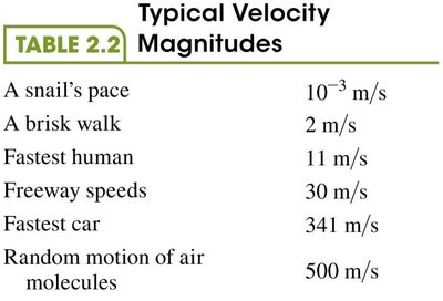
Typical Velocity Magnitudes

Velocity magnitudes vary widely depending on the context, from slow-moving objects to fast-moving particles.

Object	Velocity (m/s)
A snail's pace	$10^{-3}$
A brisk walk	2
Fastest human	11
Freeway speeds	30
Fastest car	341
Random motion of air molecules	500
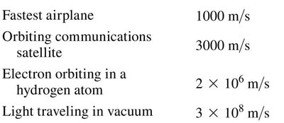
Fastest airplane	1000
Orbiting communications satellite	3000
Electron orbiting in a hydrogen atom	$2 \times 10^6$
Light traveling in vacuum	$3 \times 10^8$

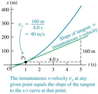
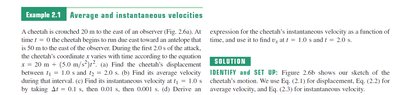
Instantaneous Velocity

Instantaneous velocity is the velocity at a specific instant, defined as the slope of the tangent to the x-t curve at that point.

• Mathematical Definition: $v_x = \lim_{\Delta t \to 0} \frac{\Delta x}{\Delta t}$

• Graphical Interpretation: The slope of the tangent line at a point on the x-t graph gives the instantaneous velocity.

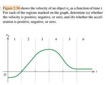
Velocity-Time Graphs

Velocity-time (vx-t) graphs provide information about the velocity at each instant and can be used to determine acceleration.

• Positive Slope: Indicates increasing velocity (speeding up).

• Negative Slope: Indicates decreasing velocity (slowing down).

• Zero Slope: Indicates constant velocity.

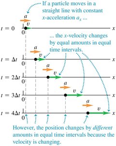
Motion Diagrams and x-t Graphs

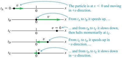
Motion diagrams visually represent the position and velocity of a particle at different times, helping to understand the direction and magnitude of motion.

• Arrows: Indicate direction and speed of motion.

• Position Markers: Show the location of the particle at each time interval.

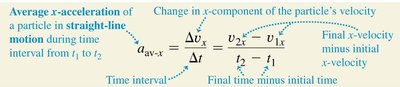
Average and Instantaneous Acceleration

Acceleration describes the rate of change of velocity with time. Average acceleration is calculated over a time interval, while instantaneous acceleration is the value at a specific instant.

• Average Acceleration (aav-x): $a_{\text{av-x}} = \frac{\Delta v_x}{\Delta t} = \frac{v_{x2} - v_{x1}}{t_2 - t_1}$

• Instantaneous Acceleration: The slope of the tangent to the vx-t curve at a point.

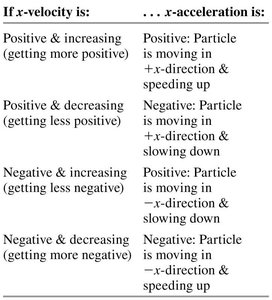
Rules for the Sign of x-Acceleration

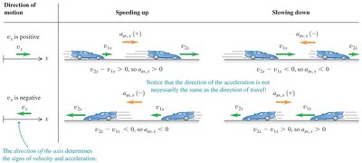
The sign of acceleration depends on the direction of velocity and whether the object is speeding up or slowing down.

If x-velocity is:	x-acceleration is:
Positive & increasing	Positive: Particle is moving in +x-direction & speeding up
Positive & decreasing	Negative: Particle is moving in +x-direction & slowing down
Negative & increasing	Positive: Particle is moving in -x-direction & slowing down
Negative & decreasing	Negative: Particle is moving in -x-direction & speeding up

Constant Acceleration and Kinematic Equations

When acceleration is constant, the motion can be described using kinematic equations. These equations relate displacement, velocity, acceleration, and time.

• Kinematic Equations:

  • $v_x = v_{0x} + a_x t$

  • $x = x_0 + v_{0x} t + \frac{1}{2} a_x t^2$

  • $v_x^2 = v_{0x}^2 + 2 a_x (x - x_0)$

  • $x - x_0 = \frac{1}{2} (v_{0x} + v_x) t$

• Application: These equations are used to solve problems involving motion with constant acceleration, such as a car accelerating along a highway or a motorcycle speeding up after leaving city limits.

Graphical Representation of Constant Acceleration

Graphs of position, velocity, and acceleration versus time illustrate the effects of constant acceleration.

• x vs t: Parabolic curve for constant acceleration.

• vx vs t: Linear graph; slope equals acceleration.

• ax vs t: Horizontal line; area under curve gives change in velocity.

Summary Table: Kinematic Equations and Quantities

The following table summarizes the kinematic equations and the quantities they include:

Equation	Includes Quantities
$v_x = v_{0x} + a_x t$	t, v_x, a_x
$x = x_0 + v_{0x} t + \frac{1}{2} a_x t^2$	t, x, a_x
$v_x^2 = v_{0x}^2 + 2 a_x (x - x_0)$	x, v_x, a_x
$x - x_0 = \frac{1}{2} (v_{0x} + v_x) t$	t, v_x

Example Problems

Worked examples illustrate the application of kinematic equations to real-world scenarios, such as calculating the position and velocity of a motorcycle or car under constant acceleration.

• Example: A motorcyclist accelerates at 4.0 m/s2 from an initial velocity of 15 m/s. After 2.0 s, the position and velocity can be found using: $x = x_0 + v_{0x} t + \frac{1}{2} a_x t^2$ $v_x = v_{0x} + a_x t$

Summary

Motion along a straight line is characterized by displacement, velocity, and acceleration. Position-time and velocity-time graphs, along with kinematic equations, provide powerful tools for analyzing and predicting the motion of objects in one dimension.

Additional info: The notes include expanded explanations, definitions, and examples to ensure completeness and academic quality for exam preparation.