Motion Along a Straight Line: Kinematics in One Dimension

Motion Along a Straight Line (1D Kinematics)

Introduction to Kinematics

Kinematics is the branch of physics that describes the motion of objects without considering the causes of motion. In this chapter, we focus on motion along a straight line (the x-axis), introducing key concepts such as displacement, velocity, and acceleration.

Displacement, Time, and Average Velocity

Displacement is the change in position of a particle along a straight line. It is a vector quantity, having both magnitude and direction. The average velocity is defined as the displacement divided by the time interval over which the displacement occurs:

$v_\mathrm{av-x} = \frac{\Delta x}{\Delta t} = \frac{x_2 - x_1}{t_2 - t_1}$

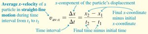
• Displacement (\(\Delta x\)): Final position minus initial position.

• Time interval (\(\Delta t\)): Final time minus initial time.

• Average velocity can be positive or negative, depending on direction.

Rules for the Sign of Velocity

The sign of velocity indicates direction along the x-axis. Positive velocity means motion in the positive x-direction; negative velocity means motion in the negative x-direction.

Average Velocity in Context

In competitive scenarios, such as a swimming race, the winner is the one with the greatest magnitude of average velocity, not necessarily the one who moves fastest at any instant.

Position-Time Graphs

A position-time (x-t) graph visually represents how an object's position changes over time. The slope of the line connecting two points on the graph gives the average velocity over that interval.

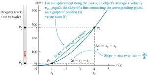
• Slope = Average velocity: $\text{Slope} = \frac{\Delta x}{\Delta t}$

Instantaneous Velocity

Instantaneous velocity is the velocity of a particle at a specific instant. It is the limit of the average velocity as the time interval approaches zero:

$v_x = \lim_{\Delta t \to 0} \frac{\Delta x}{\Delta t} = \frac{dx}{dt}$

• Instantaneous velocity equals the slope of the tangent to the x-t curve at a point.

• Average speed is not the magnitude of average velocity if the path is not straight.

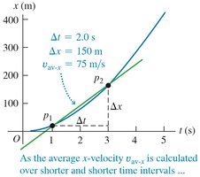
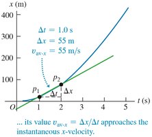
Finding Velocity on an x-t Graph

As the time interval used to calculate average velocity becomes smaller, the average velocity approaches the instantaneous velocity at a point.

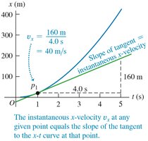
Interpreting x-t Graphs

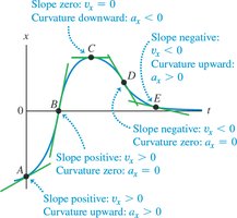
The slope of the x-t graph at any point gives the instantaneous velocity. Positive slope means positive velocity, negative slope means negative velocity, and zero slope means the object is momentarily at rest.

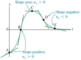
Motion Diagrams

Motion diagrams use a series of images or vectors to represent an object's position and velocity at successive times, helping visualize changes in motion.

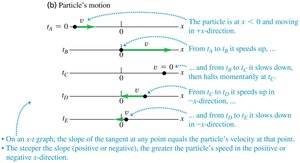
Acceleration

Average Acceleration

Acceleration describes how velocity changes with time. The average acceleration is defined as the change in velocity divided by the time interval:

$a_\mathrm{av-x} = \frac{\Delta v_x}{\Delta t} = \frac{v_{2x} - v_{1x}}{t_2 - t_1}$

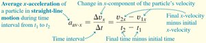
• Acceleration is a vector; its sign indicates direction of velocity change.

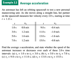
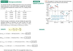
Example: Calculating Average Acceleration

Consider an astronaut's velocity measured at different times. The average acceleration over each interval can be calculated using the formula above.

Instantaneous Acceleration

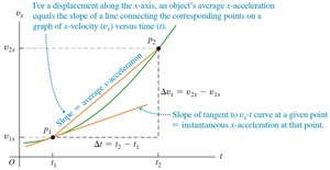
Instantaneous acceleration is the rate at which velocity changes at a specific instant:

$a_x = \lim_{\Delta t \to 0} \frac{\Delta v_x}{\Delta t} = \frac{dv_x}{dt}$

• Instantaneous acceleration equals the slope of the tangent to the vx-t curve at a point.

Finding Acceleration on a vx-t Graph

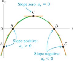
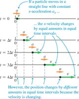
The slope of a velocity-time graph gives the acceleration. A straight line indicates constant acceleration; a curved line indicates changing acceleration.

Motion Diagrams for Acceleration

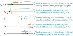
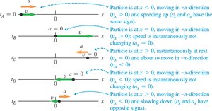
Motion diagrams can also illustrate acceleration, showing how velocity vectors change in magnitude and direction over time.

Rules for the Sign of Acceleration

The sign of acceleration indicates whether the object is speeding up or slowing down, and in which direction. If velocity and acceleration have the same sign, the object speeds up; if opposite, it slows down.

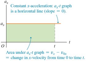
Analyzing x-t and vx-t Graphs

By examining the curvature and slope of x-t and vx-t graphs, one can determine the sign and magnitude of velocity and acceleration at various points.

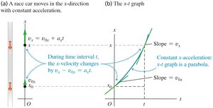
Equations of Motion with Constant Acceleration

When acceleration is constant, the following equations describe the motion of an object along a straight line:

Equation	Includes Quantities
$v_x = v_{0x} + a_x t$	t, $v_x$, $a_x$
$x = x_0 + v_{0x} t + \frac{1}{2} a_x t^2$	t, x, $a_x$
$v_x^2 = v_{0x}^2 + 2 a_x (x - x_0)$	x, $v_x$, $a_x$
$x - x_0 = \frac{1}{2} (v_{0x} + v_x) t$	x, $v_x$, t

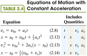
• These equations are valid only for constant acceleration.

Freely Falling Objects

Definition and Characteristics

Free fall refers to the motion of objects under the influence of gravity alone, with negligible air resistance. The acceleration due to gravity near Earth's surface is $g = 9.8\ \mathrm{m/s^2}$ downward.

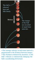
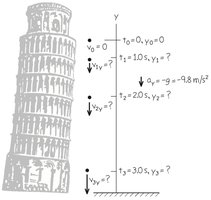
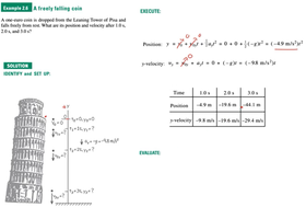
Example: A Freely Falling Coin

For an object dropped from rest, the equations of motion can be used to find its position and velocity at any time:

• Initial velocity $v_0 = 0$

• Acceleration $a = -g$ (downward)

Up-and-Down Motion in Free Fall

When an object is thrown upward, it slows down under gravity, stops momentarily at the highest point, and then accelerates downward. The acceleration is always $-g$.

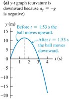
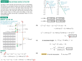
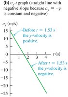
• At the highest point, velocity is zero but acceleration is still $-g$.

Velocity and Position by Integration

When acceleration is not constant, the velocity and position can be found by integrating acceleration and velocity, respectively, over time:

$v_x = \int a_x\,dt$

$x = \int v_x\,dt$

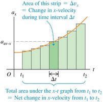
• The area under the acceleration-time graph gives the change in velocity.

• The area under the velocity-time graph gives the displacement.

Summary Table: Equations of Motion with Constant Acceleration

Equation	Variables
$v_x = v_{0x} + a_x t$	$v_x$, $v_{0x}$, $a_x$, $t$
$x = x_0 + v_{0x} t + \frac{1}{2} a_x t^2$	$x$, $x_0$, $v_{0x}$, $a_x$, $t$
$v_x^2 = v_{0x}^2 + 2 a_x (x - x_0)$	$v_x$, $v_{0x}$, $a_x$, $x$, $x_0$
$x - x_0 = \frac{1}{2} (v_{0x} + v_x) t$	$x$, $x_0$, $v_{0x}$, $v_x$, $t$

Additional info: The above notes are expanded with academic context to ensure clarity and completeness for college-level Physics with Calculus students. All equations are provided in LaTeX format for clarity. Only directly relevant images are included to reinforce key concepts.