Motion Along a Straight Line: Position-Time Graphs and Kinematics

Motion Along a Straight Line

Position-Time Graphs

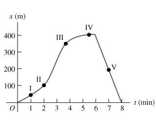
Position-time graphs are fundamental tools in physics for visualizing and analyzing the motion of objects along a straight line. The vertical axis represents position (x), while the horizontal axis represents time (t). The slope of the graph at any point gives the object's velocity, and changes in slope indicate changes in velocity (acceleration).

• Key Point 1: The slope of a position-time graph represents the velocity of the object. A steeper slope means higher velocity.

• Key Point 2: A horizontal segment indicates the object is stationary (zero velocity).

• Key Point 3: A curve indicates changing velocity, i.e., acceleration or deceleration.

• Key Point 4: Negative slope indicates motion in the opposite direction.

• Example: In the first graph, the object moves forward, slows down, stops, and then moves backward, as seen by the changing slope and direction.

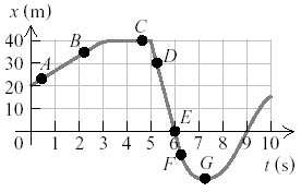
Interpreting Position-Time Graphs

To analyze position-time graphs, identify segments with constant slope (constant velocity), increasing or decreasing slope (acceleration or deceleration), and points where the slope changes sign (direction reversal).

• Key Point 1: The velocity at any instant is given by the tangent to the curve at that point.

• Key Point 2: The area under the velocity-time graph (not shown here) gives displacement, but for position-time graphs, the value at each time gives the object's location.

• Example: In the second graph, the object moves forward, stops, reverses direction, and then moves forward again.

Kinematics: Equations of Motion

Constant Acceleration

Kinematics deals with the description of motion without considering its causes. For motion with constant acceleration, the following equations are used:

• Key Point 1: The basic kinematic equations for constant acceleration are:

$x = x_0 + v_0 t + \frac{1}{2} a t^2$

$v = v_0 + a t$

$v^2 = v_0^2 + 2a(x - x_0)$

• Key Point 2: These equations relate position (x), initial position (x_0), velocity (v), initial velocity (v_0), acceleration (a), and time (t).

• Example: If a train decelerates at a constant rate, its position and velocity at any time can be calculated using these equations.

Application: Train Deceleration Problem

Consider a scenario where a train is decelerating to avoid collision with another train ahead. The diagram shows the velocities, acceleration, and distance between the trains.

• Key Point 1: The initial velocity (v_{PT}), acceleration (a), and distance (d) are given.

• Key Point 2: The equations of motion can be used to determine if the train will stop in time or collide.

• Example: Using $x = x_0 + v_0 t + \frac{1}{2} a t^2$ and $v = v_0 + a t$, one can solve for the stopping distance and time.

Summary Table: Position-Time Graph Features

Graph Feature	Physical Meaning	Example
Positive Slope	Object moving forward	Segment I-II in image_1
Zero Slope	Object stationary	Segment III-IV in image_1
Negative Slope	Object moving backward	Segment IV-V in image_1
Changing Slope	Acceleration or deceleration	Segments II-III, D-E in image_2

Additional info: Academic context and explanations have been expanded to ensure completeness and clarity for exam preparation.