Motion Graphs and Kinematics: Study Notes for College Physics

Representing Motion

Motion Diagrams

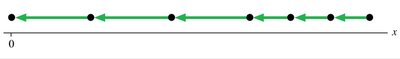
Motion diagrams are visual representations of an object's movement over time, typically showing position at successive time intervals. They help us understand direction, speed, and changes in velocity.

• Key Point 1: Each dot represents the object's position at a specific time.

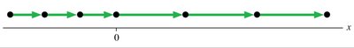
• Key Point 2: Arrows indicate the direction and magnitude of velocity.

• Example: A car moving west with decreasing velocity is shown by shorter arrows pointing left.

• Example: A car moving east with constant velocity is shown by equal-length arrows pointing right.

Motion in One Dimension

Position-Time, Velocity-Time, and Acceleration-Time Graphs

Graphs are essential tools for representing motion quantitatively. The horizontal axis is always time (t), while the vertical axis can be position (x), velocity (v), or acceleration (a).

• Key Point 1: x-t graphs show how position changes over time.

• Key Point 2: v-t graphs show how velocity changes over time.

• Key Point 3: a-t graphs show how acceleration changes over time.

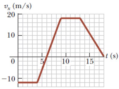
• Example: The velocity-time graph below shows a car accelerating, moving at constant velocity, then decelerating.

Interpreting Motion Graphs

Understanding the relationships between position, velocity, and acceleration graphs is crucial for analyzing motion.

• Key Point 1: The slope of the x-t graph gives velocity; the slope of the v-t graph gives acceleration.

• Key Point 2: The area under the v-t graph gives displacement.

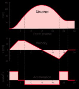
• Example: The following set of graphs shows distance, velocity, and acceleration for a moving object.

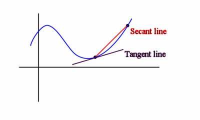
Secant and Tangent Lines

Secant and tangent lines are used to find average and instantaneous rates of change, respectively.

• Key Point 1: Secant line: Connects two points on a graph; its slope gives the average rate of change.

• Key Point 2: Tangent line: Touches the graph at one point; its slope gives the instantaneous rate of change.

• Example: The diagram below illustrates secant and tangent lines on a curve.

Kinematic Equations for Constant Acceleration

Algebraic Description of Motion

For constant acceleration, motion can be described using kinematic equations. These equations relate position, velocity, acceleration, and time.

• Key Point 1: The following are the kinematic equations for constant acceleration:

  • $v_f = v_i + a t$

  • $x_f = x_i + v_i t + \frac{1}{2} a t^2$

  • $v_f^2 = v_i^2 + 2 a (x_f - x_i)$

  • $\Delta x = \frac{v_f + v_i}{2} t$

• Key Point 2: These equations are used to solve problems involving position, velocity, and acceleration.

• Example: A car slows down from 75 km/h to 40 km/h over a distance of 50 m. Find its acceleration using $v_f^2 = v_i^2 + 2 a \Delta x$.

Special Case: Freely Falling Objects

Objects in free fall experience constant acceleration due to gravity, $g = 9.8 \frac{m}{s^2}$, directed toward the Earth's surface.

• Key Point 1: The acceleration is independent of mass.

• Key Point 2: The sign of $a$ depends on the chosen axis direction.

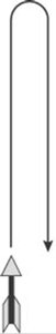
• Example: An arrow launched vertically upward follows a trajectory affected only by gravity.

Problem Solving in Kinematics

Steps for Solving Kinematics Problems

Organized problem solving is essential for success in physics. Follow these steps:

1. Draw a diagram to visualize the situation.

2. List knowns and unknowns (identify given values and what you need to find).

3. Select the appropriate equation based on the variables involved.

4. Plug in numbers and units carefully.

5. Calculate the answer.

6. Display the answer with units and box it for clarity.

Graphical Analysis of Motion

Common Velocity-Time Graphs

Different shapes of velocity-time graphs correspond to different types of motion.

• Key Point 1: Horizontal lines indicate constant velocity.

• Key Point 2: Sloped lines indicate constant acceleration.

• Key Point 3: Curved lines indicate changing acceleration.

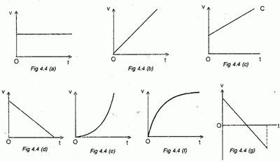
• Example: The following table summarizes common velocity-time graph shapes:

  Graph Shape	Type of Motion
  Horizontal line	Constant velocity
  Upward sloped line	Constant positive acceleration
  Downward sloped line	Constant negative acceleration
  Curved upward	Increasing acceleration
  Curved downward	Decreasing acceleration

  

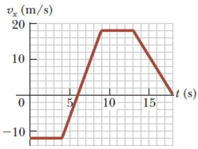
Area Under Velocity-Time Graph

The area under a velocity-time graph represents the object's displacement. Areas below the time axis are negative, corresponding to motion in the opposite direction.

• Key Point 1: Displacement is the net change in position.

• Key Point 2: Total distance traveled is the sum of all areas, regardless of sign.

• Example: Calculating displacement from a v-t graph.

Conceptual Questions

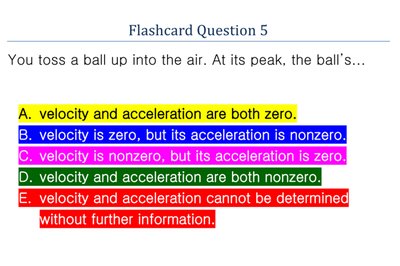
Velocity and Acceleration at the Peak of Projectile Motion

When a ball is tossed upward, at its peak, its velocity is zero but its acceleration is nonzero (equal to gravity).

• Key Point 1: Velocity is zero at the peak.

• Key Point 2: Acceleration is still $-9.8 \frac{m}{s^2}$ due to gravity.

• Example: Flashcard question about velocity and acceleration at the peak.

Summary Table: Kinematic Equations

Equation	Variables	Use
$v_f = v_i + a t$	Final velocity, initial velocity, acceleration, time	Find final velocity
$x_f = x_i + v_i t + \frac{1}{2} a t^2$	Final position, initial position, initial velocity, acceleration, time	Find position after time
$v_f^2 = v_i^2 + 2 a (x_f - x_i)$	Final velocity, initial velocity, acceleration, displacement	Find velocity or displacement
$\Delta x = \frac{v_f + v_i}{2} t$	Displacement, initial and final velocity, time	Find displacement

Additional info:

• Some context and explanations were inferred for clarity and completeness.

• All equations are provided in LaTeX format for easy reference.