Representing Motion: Position, Velocity, and Acceleration in One Dimension

Representing Motion

Coordinate Systems and Position

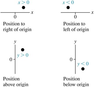
To analyze motion, we use coordinate axes to define positions in space. The x-axis is typically used for horizontal motion (positive to the right), and the y-axis for vertical motion (positive upward). The choice of axes is flexible, but must be clearly indicated in your work.

• Position is the location of an object relative to an origin (0 point) on the chosen axis.

• Positions to the right (x > 0) or above (y > 0) the origin are positive; to the left (x < 0) or below (y < 0) are negative.

Motion Diagrams

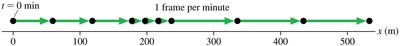
A motion diagram visually represents an object's position at successive time intervals. Each dot marks the object's location at a specific time, and arrows indicate direction and relative speed.

• Equally spaced dots: constant velocity.

• Increasing spacing: speeding up.

• Decreasing spacing: slowing down.

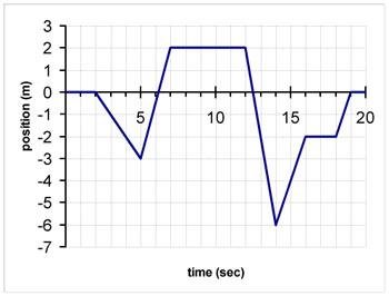
Position vs. Time Graphs

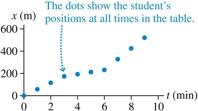
A position-versus-time graph plots an object's position (x) on the vertical axis against time (t) on the horizontal axis. This graph provides a visual summary of how position changes over time.

• The slope of the graph at any point indicates the object's velocity.

• Straight lines: constant velocity.

• Curved lines: changing velocity (acceleration).

From Position to Velocity

Understanding Slope and Velocity

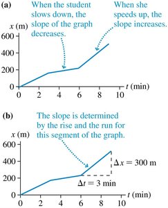
The slope of a position-versus-time graph is a key concept in kinematics. It tells us how quickly position changes with time, which is the definition of velocity.

• Average velocity ($v_{av}$) is the total displacement divided by the total time interval:

$v_{av} = \frac{\Delta x}{\Delta t} = \frac{x_f - x_i}{t_f - t_i}$

• Velocity is a vector (it has both magnitude and direction).

• SI units: meters per second (m/s).

Graphical Interpretation

On a position-time graph:

• A steeper slope means a higher speed.

• A positive slope means motion in the positive direction; a negative slope means motion in the negative direction.

• Horizontal segments (slope = 0) indicate the object is at rest.

Worked Example: Calculating Velocity from a Graph

Given a position vs. time graph, the velocity at a specific time is the slope at that point. For example, if a skateboard's position changes from 0 m to 10 m in 4 seconds, the average velocity is:

$v_{av} = \frac{10\,\text{m} - 0\,\text{m}}{4\,\text{s} - 0\,\text{s}} = 2.5\,\text{m/s}$

Negative slopes indicate negative velocity (motion in the opposite direction).

Analyzing Position vs. Time Graphs

Key Features and Interpretation

• Above the x-axis: positive position.

• Below the x-axis: negative position.

• Straight line: constant velocity.

• Curved line: changing velocity (acceleration).

• Points where the graph is flat (slope = 0): object is at rest.

Summary Table: Reading Position vs. Time Graphs

Graph Feature	Physical Meaning
Above x-axis	Positive position
Below x-axis	Negative position
Straight line	Constant velocity
Horizontal line	At rest
Curved line	Changing velocity (acceleration)

From Position to Velocity: Velocity-Time Graphs

Constructing Velocity-Time Graphs

A velocity-versus-time graph can be deduced from the slope of the position-versus-time graph. It provides another way to represent an object's motion.

• Constant velocity: horizontal line.

• Changing velocity: sloped or curved line.

Example: Matching Motion Diagrams and Velocity Graphs

Given a motion diagram, the corresponding velocity-time graph shows how the object's speed and direction change over time.

From Velocity to Position: Area Under the Curve

Displacement from Velocity-Time Graphs

The displacement ($\Delta x$) of an object is equal to the area under the velocity-time graph during a given time interval ($\Delta t$):

$\Delta x = \text{Area under } v(t) \text{ curve}$

• For constant velocity, this area is a rectangle: $\Delta x = v \cdot \Delta t$.

• For changing velocity, sum the areas of geometric shapes under the curve.

Instantaneous Velocity

Definition and Calculation

Instantaneous velocity is the velocity of an object at a specific instant in time. It is found as the slope of the tangent to the position-time curve at that point.

• For a curve $x(t)$, the instantaneous velocity at time $t$ is:

$v = \lim_{\Delta t \to 0} \frac{\Delta x}{\Delta t} = \frac{dx}{dt}$

• Graphically, draw a tangent line at the point of interest and calculate its slope.

Velocity Changing with Time: Acceleration

Average and Instantaneous Acceleration

Acceleration describes how velocity changes with time. The average acceleration ($a_{av}$) is given by:

$a_{av} = \frac{\Delta v}{\Delta t} = \frac{v_f - v_i}{t_f - t_i}$

• Acceleration is a vector (direction matters).

• SI units: meters per second squared (m/s2).

• "Speeding up" or "slowing down" depends on the direction of velocity and acceleration.

Worked Example: Lion's Acceleration

A lion accelerates from rest ($v_i = 0$) at $a = 9.5\,\text{m/s}^2$ to $v_f = 4.5\,\text{m/s}$. The time required is:

$t = \frac{v_f - v_i}{a} = \frac{4.5\,\text{m/s} - 0}{9.5\,\text{m/s}^2} \approx 0.47\,\text{s}$

Worked Example: Skater with Constant Acceleration

A skater moves east at $3.20\,\text{m/s}$ and experiences a constant acceleration of $0.8\,\text{m/s}^2$ westward. To find the final velocity after $3.0\,\text{s}$:

$v_f = v_i + a t = 3.20\,\text{m/s} + (-0.8\,\text{m/s}^2)(3.0\,\text{s}) = 0.8\,\text{m/s}$

• After $6.0\,\text{s}$, $v_f = 3.20 - 0.8 \times 6.0 = -1.6\,\text{m/s}$ (now moving west).

Plotting velocity vs. time and position vs. time graphs helps visualize the motion and identify intervals of speeding up or slowing down.

Summary Table: Key Kinematic Quantities

Quantity	Definition	SI Unit
Position ($x$)	Location relative to origin	meter (m)
Displacement ($\Delta x$)	Change in position	meter (m)
Velocity ($v$)	Rate of change of position	meter/second (m/s)
Acceleration ($a$)	Rate of change of velocity	meter/second2 (m/s2)