Addition Rule and Complements in Probability

5.2 The Addition Rule and Complements

Addition Rule for Disjoint Events

The Addition Rule is a fundamental concept in probability that allows us to calculate the probability of the union of two or more events. When events are disjoint (also called mutually exclusive), they have no outcomes in common.

• Disjoint Events: Events that cannot occur at the same time. For example, drawing a chip labeled '2' and a chip labeled '8' from a bag in a single draw are disjoint events.

• Addition Rule for Disjoint Events: If events E, F, G, ... are disjoint, then: $P(E \text{ or } F \text{ or } G \text{ or } \ldots) = P(E) + P(F) + P(G) + \ldots$

Example: Suppose the probability model for the number of rooms in a housing unit is as follows:

Number of Rooms	Probability
One	0.010
Two	0.032
Three	0.093
Four	0.176
Five	0.219
Six	0.189
Seven	0.122
Eight	0.079
Nine or more	0.080

• Probability of two or three rooms: $P(\text{Two or Three}) = P(\text{Two}) + P(\text{Three}) = 0.032 + 0.093 = 0.125$

• Probability of one, two, or three rooms: $P(\text{One or Two or Three}) = 0.010 + 0.032 + 0.093 = 0.135$

Note: Always verify that the sum of all probabilities in a probability model equals 1.

Addition Rule for Non-Disjoint Events (General Addition Rule)

When two events are not disjoint (i.e., they can occur together), the Addition Rule must be adjusted to avoid double-counting the outcomes they share.

• General Addition Rule: $P(E \text{ or } F) = P(E) + P(F) - P(E \text{ and } F)$

• This formula subtracts the probability of the intersection (both events occurring) to correct for double-counting.

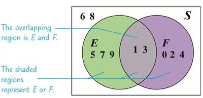
Example: Suppose E = "choose an odd number" and F = "choose a number less than or equal to 4" from chips labeled 0–9. E = {1,3,5,7,9}, F = {0,1,2,3,4}. The outcomes 1 and 3 are in both E and F.

• Total outcomes in E or F: 8

• Total outcomes in sample space: 10

• $P(E \text{ or } F) = \frac{8}{10} = 0.8$

• Alternatively, using the formula: $P(E) = 0.5$, $P(F) = 0.5$, $P(E \text{ and } F) = 0.2$ $P(E \text{ or } F) = 0.5 + 0.5 - 0.2 = 0.8$

Example: If $P(E) = 0.32$, $P(F) = 0.61$, and $P(E \text{ and } F) = 0.10$, then: $P(E \text{ or } F) = 0.32 + 0.61 - 0.10 = 0.83$

If E and F are mutually exclusive, $P(E \text{ and } F) = 0$, so $P(E \text{ or } F) = 0.32 + 0.61 = 0.93$.

Addition Rule with Contingency Tables

Contingency tables (or two-way tables) organize data into categories and are useful for calculating probabilities involving two categorical variables.

	Males (millions)	Females (millions)
Never Married	45.3	40.1
Married	68.5	69.3
Widowed	3.5	11.4
Divorced	10.7	14.8

• Probability a resident is male: $P(\text{Male}) = \frac{\text{Total males}}{\text{Total population}}$

• Probability a resident is widowed: $P(\text{Widowed}) = \frac{\text{Total widowed}}{\text{Total population}}$

• Probability a resident is widowed or divorced: $P(\text{Widowed or Divorced}) = P(\text{Widowed}) + P(\text{Divorced})$ (since these are disjoint)

• Probability a resident is male or widowed: Use the general addition rule: $P(\text{Male or Widowed}) = P(\text{Male}) + P(\text{Widowed}) - P(\text{Male and Widowed})$

Complement Rule

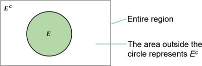
The complement of an event E, denoted as $E^c$, consists of all outcomes in the sample space that are not in E. The probability of the complement is:

• $P(E^c) = 1 - P(E)$

Example: If 31.6% of households own a dog, the probability that a randomly selected household does not own a dog is: $P(\text{No dog}) = 1 - 0.316 = 0.684$

Using the Complement Rule with Frequency Tables

Frequency tables can be used to calculate probabilities for events and their complements.

Travel Time	Frequency
Less than 5 minutes	24,358
5 to 9 minutes	39,112
10 to 14 minutes	62,124
15 to 19 minutes	72,854
20 to 24 minutes	74,386
25 to 29 minutes	30,099
30 to 34 minutes	45,043
35 to 39 minutes	11,169
40 to 44 minutes	8,045
45 to 59 minutes	15,650
60 to 89 minutes	5,451
90 or more minutes	4,895

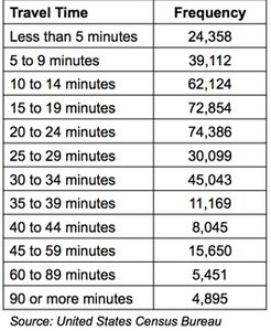
• Probability of 90 or more minutes: $P(\text{90 or more}) = \frac{4,895}{\text{Total}}$

• Probability of less than 90 minutes: $P(\text{Less than 90}) = 1 - P(\text{90 or more})$

Additional info: To find the total, sum all frequencies in the table.