Binomial Probability Distributions: Concepts, Calculations, and Applications

Binomial Probability Distributions

Definition and Properties of Binomial Experiments

A binomial experiment is a probability experiment that meets specific criteria, making it suitable for analysis using the binomial probability distribution. These experiments are foundational in statistics for modeling scenarios with two possible outcomes per trial.

• Fixed Number of Trials (n): The experiment consists of a predetermined number of trials.

• Independence: Each trial is independent of the others.

• Two Outcomes: Each trial results in one of two outcomes, commonly labeled as "success" or "failure."

• Constant Probability: The probability of success, denoted as p, remains the same for each trial. The probability of failure is q = 1 - p.

• Random Variable (x): The variable of interest, x, counts the number of successes in the n trials.

Notation:

• n: Number of trials

• p: Probability of success on a single trial

• q: Probability of failure on a single trial (q = 1 - p)

• x: Number of successes in n trials

Identifying Binomial Experiments

To determine if a scenario is a binomial experiment, check if it satisfies all the binomial properties. For example, drawing a card from each of several well-shuffled decks and recording a specific outcome (e.g., face card or not) is binomial if each draw is independent and the probability remains constant.

• Example: Drawing one card from each of 6 independent decks and recording if it is a face card. Here, n = 6, p = 12/52 (since there are 12 face cards in a deck), q = 40/52, and x is the number of face cards drawn.

Calculating Binomial Probabilities

Calculating the probability of a specific number of successes can be done using the Multiplication Rule or, more efficiently, the Binomial Probability Formula. For small n, a tree diagram can help visualize all possible outcomes.

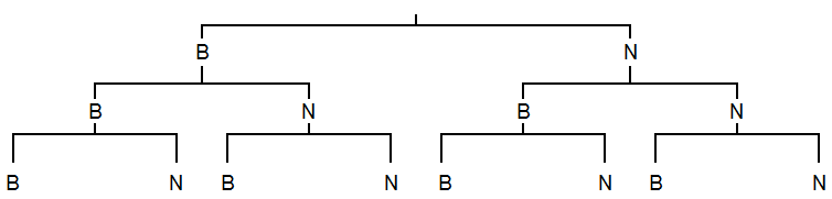
• Example: Probability that exactly 1 out of 3 households has a Blu-ray player, with p = 1/5 and q = 4/5. List all possible outcomes and sum the probabilities for those with exactly one Blu-ray.

The Binomial Probability Formula

The binomial probability formula provides a shortcut for calculating the probability of exactly x successes in n independent trials:

$P(x) = \binom{n}{x} p^x q^{n-x}$

• n: Number of trials

• x: Number of successes

• p: Probability of success

• q: Probability of failure

• \binom{n}{x}: Number of ways to choose x successes from n trials ("n choose x")

Example: For n = 3, x = 1, p = 1/5, q = 4/5:

$P(1) = \binom{3}{1} \left(\frac{1}{5}\right)^1 \left(\frac{4}{5}\right)^{2} = 3 \times \frac{1}{5} \times \frac{16}{25} = \frac{48}{125}$

Constructing Binomial Probability Distributions

A binomial probability distribution lists the probability for each possible value of the random variable x (number of successes). This is useful for understanding the likelihood of different outcomes in a binomial experiment.

• Example: If 10% of balloons are defective and you buy 8, the probability distribution for the number of defective balloons is calculated for x = 0 to 8 using the binomial formula.

x	P(x)
0	0.43046721
1	0.38263752
2	0.14880348
3	0.03306744
4	0.00459270
5	0.00040824
6	0.00002268
7	0.00000072
8	0.00000001

Using Technology for Binomial Calculations

Calculators such as the TI-83/84 can quickly compute binomial probabilities and distributions using built-in functions like binompdf (for individual probabilities) and binomcdf (for cumulative probabilities).

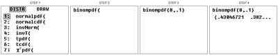
• binompdf(n, p): Computes the probability distribution for all x values.

• binomcdf(n, p, x): Computes the cumulative probability for x or fewer successes.

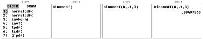
Cumulative Binomial Probabilities and Complements

To find the probability of "no more than x" successes, sum the probabilities for all values up to x (cumulative probability). For "more than x," subtract the cumulative probability from 1.

• Example: Probability that no more than 3 balloons are defective: $P(x \leq 3) = P(0) + P(1) + P(2) + P(3)$

• Complement: Probability that more than 3 are defective: $P(x > 3) = 1 - P(x \leq 3)$

Graphing Binomial Probability Distributions

Binomial probability distributions can be visualized using histograms, where the x-axis represents the number of successes and the y-axis represents the probability of each outcome.

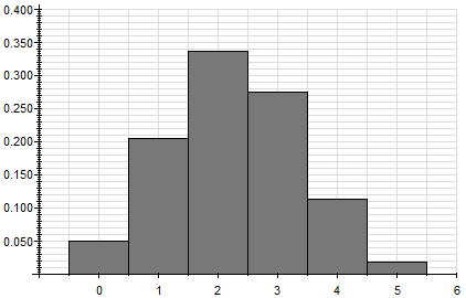
• Example: For n = 5, p = 0.45, the histogram shows the probabilities for x = 0 to 5 successes.

Population Parameters for Binomial Distributions

The mean, variance, and standard deviation of a binomial distribution can be calculated using the following formulas:

• Mean: $\mu = n p$

• Variance: $\sigma^2 = n p q$

• Standard Deviation: $\sigma = \sqrt{n p q}$

Example: For n = 20, p = 0.41, q = 0.59:

• Mean: $\mu = 20 \times 0.41 = 8.2$

• Variance: $\sigma^2 = 20 \times 0.41 \times 0.59 = 4.838$

• Standard Deviation: $\sigma = \sqrt{4.838} \approx 2.2$

Summary Table: Key Properties of Binomial Experiments

Property	Description
Number of Trials (n)	Fixed and known in advance
Independence	Each trial does not affect the others
Outcomes	Exactly two (success/failure)
Probability of Success (p)	Constant for each trial
Random Variable (x)	Counts number of successes

Additional info: The binomial distribution is widely used in quality control, survey analysis, and reliability engineering, wherever the outcome of interest is the count of successes in repeated, independent trials.