Binomial Probability Distributions: Concepts, Calculations, and Applications

Binomial Probability Distributions

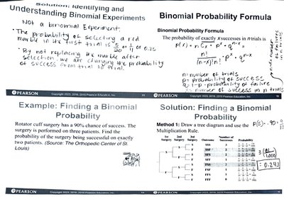
Understanding Binomial Experiments

A binomial experiment is a probability experiment that satisfies specific criteria. Recognizing these criteria is essential for determining when to use binomial probability methods.

• Fixed Number of Trials (n): The experiment is repeated a set number of times.

• Independent Trials: Each trial is independent of the others.

• Two Possible Outcomes: Each trial results in either a success or a failure.

• Constant Probability (p): The probability of success remains the same for each trial.

• Random Variable (X): Counts the number of successes in n trials, where $X = 0, 1, 2, ..., n$.

Example: A doctor performs a surgical procedure with an 85% success rate on eight patients. Here, n = 8, p = 0.85, q = 0.15, and X can take values from 0 to 8.

Non-Binomial Example: Drawing marbles from a jar without replacement is not a binomial experiment because the probability of success changes after each draw, violating the independence and constant probability conditions.

Notation for Binomial Experiments

• n: Number of trials

• p: Probability of success in a single trial

• q: Probability of failure in a single trial ($q = 1 - p$)

• X: Random variable representing the number of successes in n trials

Binomial Probability Formula

The probability of obtaining exactly x successes in n independent trials is given by the binomial probability formula:

$P(x) = \frac{n!}{x!(n-x)!} p^x q^{n-x}$

• $n!$ denotes the factorial of n.

• $p$ is the probability of success, $q$ is the probability of failure.

• $x$ is the number of successes (where $0 \leq x \leq n$).

Example: For three surgeries with a 90% success rate, the probability of exactly two successes is calculated as:

$P(2) = \frac{3!}{2!1!} (0.9)^2 (0.1)^1 = 3 \times 0.81 \times 0.1 = 0.243$

Finding Binomial Probabilities Using Technology

Technology such as statistical calculators or software can be used to compute binomial probabilities efficiently, especially for large n.

• For example, using a TI-84 calculator: binompdf(n, p, x) computes $P(X = x)$.

• Example: In a survey, 75% of adults experience digital device fatigue. For 100 randomly selected adults, the probability that exactly 66 experience fatigue is found using binompdf(100, 0.75, 66), yielding approximately 0.011.

Interpretation: If the probability of an event is less than 0.05, it is considered unusual.

Finding Binomial Probabilities Using Formulas

When technology is unavailable, use the binomial formula to compute probabilities for various scenarios:

• Exactly x successes: Use the formula directly.

• At least x successes: Sum probabilities from x to n: $P(X \geq x) = P(x) + P(x+1) + ... + P(n)$

• Fewer than x successes: Sum probabilities from 0 to x-1: $P(X < x) = P(0) + P(1) + ... + P(x-1)$

Example: If 22% of adults say the economy is the most important issue, for 4 adults, the probability that exactly 2 say yes is:

$P(2) = \frac{4!}{2!2!} (0.22)^2 (0.78)^2 = 6 \times 0.0484 \times 0.6084 \approx 0.177$

Finding Binomial Probabilities Using a Table

Binomial probability tables provide precomputed probabilities for various values of n, p, and x. These are useful for quick reference when n is not too large.

• Example: If 5% of workers commute by public transportation, for 8 workers, the probability that exactly 3 use public transportation is found in the table for n = 8, p = 0.05, x = 3, yielding 0.005.

Mean, Variance, and Standard Deviation of a Binomial Distribution

The mean, variance, and standard deviation of a binomial distribution are calculated as follows:

• Mean (μ): $\mu = np$

• Variance (σ²): $\sigma^2 = npq$

• Standard Deviation (σ): $\sigma = \sqrt{npq}$

Example: In Pittsburgh, about 56% of days in June are cloudy. For 30 days, the mean number of cloudy days is $30 \times 0.56 = 16.8$, variance is $30 \times 0.56 \times 0.44 = 7.4$, and standard deviation is $\sqrt{7.4} \approx 2.7$.

Additional info: The notes above cover the essential aspects of binomial probability distributions, including identification, calculation methods, and interpretation of results. These concepts are foundational for understanding discrete probability distributions in statistics.